This article presents the most comprehensive study to date from the U.S. Bureau of Labor Statistics (BLS) to document the extent of chain drift in the Chained Consumer Price Index for All Urban Consumers (C-CPI-U). We apply various formulas to real data collected from December 1999 through December 2017 that BLS used to calculate the “official” Consumer Price Index (CPI) during that period.1 Building on earlier work conducted by Joshua Klick, we employ unity and circularity tests as well as multilateral index comparisons to empirically assess the impact of chain drift in the top-level C-CPI-U, U.S. city average, all-items index.2 We also conduct circularity tests of the C-CPI-U, U.S. city average, indexes at the subaggregate expenditure-class level. After comparing multilateral and bilateral versions of this index, we found that chain drift adds an estimated 0.11 percent to price change in the national, all-items, chained Törnqvist index. Estimates of chain drift that are based on unity and circularity tests show similar levels of drift, but we find those test results depend on the choice of base month and exhibit strong seasonal patterns. We find more substantial drift in certain indexes at the subaggregate level, but the majority of expenditure-class indexes satisfy the circularity test approximately. We also find that a monthly chained, Laspeyres index shows substantial drift.
Background
In August 2002, the CPI program began publishing the C-CPI-U. The C-CPI-U was implemented to address concerns that the official Consumer Price Index for All Urban Consumers (CPI-U) suffered from upper-level substitution bias, given that it is calculated using a Laspeyres (technically, a Lowe) formula. As described by Robert Cage, John Greenlees, and Patrick Jackman in a 2003 conference paper, the C-CPI-U “employs a superlative Törnqvist formula and utilizes expenditure data in adjacent time periods in order to reflect the effect of any substitution that consumers make across item categories in response to changes in relative prices.”3
The Boskin Commission report submitted to the U.S. Senate Finance Committee in December 1996 estimated that the official CPI-U was biased upward by 0.15 percentage points because of consumer substitution across item categories (upper-level substitution) and that it was biased upward by 0.25 percentage points because of consumer substitution within item categories (lower-level substitution).4 Upper-level substitution refers to substitution between these categories. Lower-level substitution refers to substitution within any of 243 item categories at the lowest level of aggregation in the CPI classification scheme.
According to the Boskin Commission, “Substitution bias occurs because a fixed market basket fails to reflect the fact that consumers substitute relatively less for more expensive goods when relative prices change.”5 For the CPI-U, U.S. city average, all-items index, an example of upper-level substitution bias is when consumers substitute chicken for steak or beer for wine. An example of lower-level substitution bias is when consumers substitute low-fat milk for whole milk. “Levels” refer to the placement of categories of goods and services within the CPI aggregation structure.
The CPI-U is based on prices collected from monthly surveys—as well as alternative data sources for some item categories—and on expenditures collected from the Consumer Expenditure Surveys administered monthly during 24-month intervals between biennial expenditure-weight updates. The CPI-U thus measures the changes in prices for a market basket of goods and services that remains unchanged between biennial updates (specific items may change because of item replacement and sample rotation), with quantity data captured implicitly via lagged expenditures. Biennial updates also mean that price and quantity data are “chained” at each biennial “rebase” using a Lowe formula. A geometric mean formula is used in the official CPI-U to address lower-level substitution bias.6
In the C-CPI-U, price and quantity data are chained each month using a Törnqvist formula that calculates an index incorporating both monthly price changes and monthly expenditure changes across item categories. Because of the amount of time that is necessary to process expenditure data, C-CPI-U data are released first in preliminary form. Three months later, they are released again in their first interim form. Six months later, they are released again in their second interim form. Nine months later, they are released again in their third interim form. In these three quarterly intervals following release in preliminary form, BLS uses a constant elasticity-of-substitution formula for the initial estimates. Twelve months later, exactly a year after the preliminary release, a Törnqvist formula is used to produce the final estimates.7
By addressing potential substitution bias, the C-CPI-U is designed to be a closer approximation to a “true” cost-of-living index (COLI). Given that the implicitly derived quantities that consumers purchase are taken to be the optimal quantities on the basis of their income or wealth, COLIs, originally conceived by A. A. Konüs, are based on the economic theory of consumer demand.8 Under the standard framework, consumers maximize utility and minimize cost, given a level of wealth or income. More specifically, under “Hicksian” demand, consumers minimize the expenditures necessary to attain a given standard of living—that is, they seek to maximize their utility at the minimal cost.9 When relative prices change, the relative affordability of different goods and services changes, which affects consumers’ standard of living. The COLI is designed to measure the compensation necessary to afford the original standard of living. Consumer inflation is thus calculated as the ratio of minimum expenditures in two periods necessary to achieve the same standard of living. In the following equation, which illustrates this ratio, iIX(0,t) is the index that represents consumer inflation over the set of i goods from period 0 to t, with the basket of goods, and thus the standard of living, remaining constant; iP0 is the price of good i in period 0, iQ0 is the quantity of good i in period 0, iPt is the price of good i in period t, and iQt is the quantity of good i in period t:

However, the choice between a chained or fixed-base index presents a tradeoff between representativeness and transitivity. Indexes are “representative” when they accurately represent not only the price trend of a “market basket” of goods and services but also the composition of the “market basket” as it changes over time. As the 2004 Consumer Price Index Manual explains,
The main problem with the use of fixed base Laspeyres indices is that the period 0 fixed basket of commodities that is being priced out in period t can often be quite different from the period t basket. Thus, if there are systematic trends in at least some of the prices and quantities in the index basket, the fixed base Laspeyres price index PL(p0, pt, q0, qt) can be quite different from the corresponding fixed base Paasche price index, PP(p0, pt, q0, qt). This means that both indices are likely to be an inadequate representation of the movement in average prices over the time period under consideration.10
Christian G. Ehemann defines an index number formula as transitive if chaining from t = 1 to t = 2 and then from t = 2 to t = 3 yields the same index value for the index at t = 3 as the direct index from t = 1 to t = 3: I(p0, p1, q0, q1) * I(p1, p2, q1, q2) * I(p2, p3, q2, q3) = I(p0, p3, q0, q3). If this condition is not met, the index is nontransitive. The monthly chained Törnqvist formula used for the C-CPI-U is nontransitive and, as a result, is subject to drift.11 Frequent weight updates may lead to increased drift in nontransitive indexes. The official index—the Consumer Price Index for All Urban Consumers (CPI-U), U.S. city average, all items—is a chained index in the sense that weights are updated biennially, but it also is a fixed-base index when it is calculated between expenditure-weight updates. The C-CPI-U uses monthly chaining with monthly weight updates (when finalized) and, in principle, may be at greater risk of measurable chain drift.
We now clarify some of the terminology associated with price-index methodology. A price index can be either fixed base or chained, and it can be either bilateral or multilateral. (In this article, we use the terms “fixed base” and “direct” interchangeably.) We rely on the Consumer Price Index Manual for precise definitions of these terms. According to the Manual, the word “bilateral” refers to the assumption that a function P, or a price index number formula, P(p0, p1, q0, q1), depends only on the data pertaining to the two situations or periods being compared. For example, P is regarded as a function of the two sets of price and quantity vectors, p0, p1, q0, q1, “that are to be aggregated into a single number that summarizes the overall change in the n price ratios p1(1)/p0(1), . . . , p1(n)/p0(n).”12 “Multilateral index number theory,” however, “refers to the case where there are more than two situations whose prices and quantities need to be aggregated.”13
On the distinction between a fixed-base index and a chained index, the Manual explains that the “chain system measures the change in prices going from one period to a subsequent period using a bilateral index number formula involving the prices and quantities pertaining to the two adjacent periods. These one-period rates of change (the links in the chain) are then cumulated to yield the relative levels of prices over the entire period under consideration.” Consider, for example, a bilateral price index P. The index is “chained” if index calculation generates the following sequence:14
1, P(p0, p1, q0, q1), P(p1, p2, q1, q2).
Under a fixed-base system, however, the bilateral index number formula P “simply computes the level of prices in period t relative to the base period 0 as P(p0, pt, q0, qt).”15 As such, the fixed-base system generates the following sequence of price levels for periods 0, 1, and 2:
1, P(p0, p1, q0, q1), P(p0, p2, q0, q2).
Empirically, chain drift is often defined as the difference between the chained and fixed-base versions of a price index. Chain drift can occur when expenditure-share weight updates lag short-term price oscillations, distorting trend reversion and leading to nontransitivity in a price index. However, several factors can lead to divergence, including the representativity of the market basket of goods and services in the base period. Our analysis also indicates that choice of base month and seasonal patterns may affect the amount of drift. Gregory Kurtzon refers to divergence resulting from consumer substitution as “good” drift. Divergence resulting from nontransitivity, which can be analyzed with the unity test, is, unambiguously, “bad” drift.16
Chaining: theory and practice
In addition to the choice of index number formula, chaining an index addresses substitution bias by providing an approach for incorporating changes in quantity over time. According to F. G. Forsythe and R. F. Fowler, Francois Divisia “put forward the new concept of an index of prices based specifically on the assumption that an index of price changes over a period of time 0 to t should depend not only on prices and quantities at 0 and t but also on the movement of prices and quantities throughout the interval 0 to t. In other words, the index should depend on the path and take account of all the data relating to prices and quantities in the interval.”17 This idea has its earliest roots in the 19th-century work of Julius Lehr and Alfred Marshall, the latter introducing the principle of chaining as a way of making index formulas more representative of ongoing changes in economic activity.18 As Forsythe and Fowler write, “Marshall was concerned only with the practical problem of allowing for the introduction of new commodities into an index of prices which he thought would be greatly facilitated if the weights were changed every year and the successive yearly indices linked or chained together by simple multiplication.”19
In principle, a Divisia index perfectly captures changes in price and quantity as they occur. Because a continuous time index is not feasible, numerous discrete time-index formulas have been developed, such as the Lowe and Törnqvist formulas used for the official CPI-U and the C-CPI-U, respectively. These formulas are weighted versions of arithmetic and geometric means. The economic theory of consumer demand provides the theoretical connection between a Divisia index and a cost-of-living index.20
Forsyth and Fowler noted a tradeoff between maintaining base-period weights and using chained indexes. Chained indexes have the potential for drift but represent recent expenditure patterns. Fixed-base indexes have no drift, but the base-period consumption basket becomes less representative as consumption patterns change. Forsyth and Fowler argued that the benefits of representativity generally outweigh the relatively small drift in a Fisher index.21
The C-CPI-U combines a Törnqvist formula with monthly chaining to provide a measure of consumer inflation that reflects monthly purchases in response to monthly changes in price. The C-CPI-U is not only a measure of consumer inflation but a measure of revealed preference. One major problem that can emerge with chaining, however, is a violation of transitivity, which is one of several axiomatic properties that are desirable for indexes to have.22 An index is transitive if long-term price change calculated with updated quantity data in each incremental period is equal to long-term price change without frequent updating from a reference period to a comparison period.
More precisely, Ehemann defines an index number formula as “transitive if chaining from t = 1 to t = 2 and then from t = 2 to t = 3 gives the same index value for the index at t = 3 as the direct index from t = 1 to t = 3”:23
I(p1, p2, q1, q2) * I(p2, p3, q2, q3) = I(p1, p3, q1, q3).
A violation of the transitivity axiom could indicate that chain drift is a problem with the index choice. If indexes are transitive, they do not exhibit chain drift. Conversely, indexes that are not transitive exhibit chain drift. Indexes that exhibit chain drift diverge from their “true” long-term trend. As a result, a chained index makes an index more representative of market-basket composition (what consumers are purchasing), but often at the expense of providing an inaccurate measure of long-term inflation. Chaining can thus involve a tradeoff between representativity and transitivity.24 For any price index, the central question is whether, in any given case, the benefits of representativity are outweighed by the cost of nontransitivity (i.e., chain drift).
Bohdan J. Szulc identified “bounce” behavior in prices resulting from such factors as seasonality or price wars as a major source of drift. “Bounce” is more likely to cause drift if a “peak” or “trough” diverges from the long-term trend.25 Thus, following Kurtzon, we can imagine the prices of two goods with equal expenditure shares “bouncing” between two periods, with the price of each good either $1 or $2 in every period, generating a price relative of 2 or 1/2. In this situation, there is no long-term inflation, but, as Kurtzon states, “this index relative would give an inflation rate of 1/2(2 + 1/2) = 1.25, or 25 [percent] inflation every period.”26 Price oscillation may reflect trend reversion as competition prevents sellers from charging prices that deviate from their long-term trends as consumer substitution “puts downward pressure on prices that are comparatively high, and it may also put upward pressure on prices that are unusually low by making them attract high sales.”27 Lorraine Ivancic, Kevin J. Fox, and W. Erwin Diewert provide a similar explanation of drift:
As a result, it is not necessarily the case that prices and quantities in adjacent periods are more similar than those in periods which are not adjacent when subannual data is used. In particular, when an item goes off sale and prices return to their “regular” price, we would expect that the use of a chained superlative index would simply (more or less exactly) reverse the previous downward movement in the index and take us back to the “regular” price level. However, in practice this may not happen because when an item comes off sale, consumers are likely to purchase less than the “average” quantity of that item for some period of time until their inventories of the item have been depleted. It is only over time that the quantities sold will gradually recover to their pre-sale levels [emphasis added]. If prices do not change over the post-sale period, all reasonable indexes will show no price change over these “regular” price periods. Thus, under these conditions (i.e., where sales are apparent), chained superlative indexes will tend to have a downward drift when compared to their fixed base counterparts.28
Methodology: test for chain drift
Because chaining has the potential to make a price index more representative of consumption behavior and marketplace activity, it is of considerable interest to determine if the benefits of a more representative index are outweighed by any “drift” that causes the index to diverge from long-term price trends. In this study, we used several tests to determine the extent to which the C-CPI-U exhibits undesirable drift. We first address the second stage of index aggregation in which component indexes—which are constructed from aggregations of price observations pertaining to specific geographic areas and item categories—are combined. We then focus on subaggregate indexes at the expenditure-class level. In the CPI aggregation structure, there are 70 expenditure-class indexes, which are one level of aggregation above the “lower level” 243 item-level indexes, which, combined with 32 index areas, form 7,776 item-area, lower-level, index-area “cells,” the building blocks of CPI index construction. Item-area component indexes use fixed-weight formulas, but, like all bilateral indexes, they are effectively chained at each weight update. Every time the relative weights of price quotes change within a cell, which can occur because of subsampling and partial cell sample rotation, drift can occur.
Unity test
C. M. Walsh introduced the unity test as one method for detecting drift. As the Consumer Price Index Manual explains, this test uses “the bilateral index formula P(p0, p1, q0, q1) to calculate the change in prices going from period 0 to 1.” It then uses “the same formula evaluated at the data corresponding to periods 1 and 2, P(p1, p2, q1, q2), to calculate the change in prices going from period 1 to 2” and then uses “P(pT−1, pT, qT−1, qT) to calculate the change in prices going from period T – 1 to T.” The unity test then “introduce[s] an artificial period T + 1 that has exactly the price and quantity of the initial period 0 and use[s] P(pT, p0, qT, q0) to calculate the change in prices going from period T to 0.” In the last step, “multiply all of these indices together.”29
The unity test thus chains index formulas from point 0 to point T and sets the price and quantity in period T + 1 equal to the price and quantity observed in period 0. In the next step, I(p0, pT, q0, qT) is used to calculate the change in prices from period T to period 0. In the final step, multiply all of the chained indexes together. According to the Consumer Price Index Manual, if the result is an index value equal to the index value in period 0, “we end up where we started, [and] the product of all of these indices should ideally be one.”30 Mathematically, we have the following:
DriftUnity,t = I(p0, p1, q0, q1) * I(p1, p2, q1, q2) *…* I(pt, p0, qt, q0).
This procedure computes the chained price index until month t and then appends the initial set of prices and quantities (p0, q0) to the end of the series. Because the final period is the same as the first, a fully transitive index should show no change. We produced estimates of drift over the entire series and, iteratively, sequentially conducted this test for each period t after the base period, setting the terminal month indexes and weights equal to the exact values from the starting month iteratively from December 1999 to November 2017. Thus, in the first run of the test, we conducted an iterative unity test with December 1999 as the starting point, and each successive month up to November 2017, with December 2017 as the terminal month. Then, we ran another iterative unity test, with January 2000 as the starting point, and each successive month up to November 2017, with December 2017 as the terminal month. We repeated this process through November 2017. We also produced unity tests on indexes that are based on bounded price relatives. Monthly price changes in these indexes are capped at 95-percent declines and 2,000-percent increases.
Circularity test
The unity test, or what Diewert called the “multiperiod identity test,” is a special case of the circularity test.31 In both cases, the aim is to test whether transitivity holds. If transitivity holds, index formulas generate the same measurement of long-term price change. If it does not, fixed-base formulas and chained-index formulas diverge. Or, stated differently, chained indexes drift. Note that the Consumer Price Index Manual recommends the circularity and unity tests not as measures for deciding whether to use fixed-base or chained indexes, but as measures of “how ‘good’ a particular index number formula is.”32 Drift is also a reason why the Manual recommends chaining for series that have smooth trends. As the Manual notes, Alterman, Diewert, and Feenstra “show that if the logarithmic price ratios ln( ) trend linearly with time t and the expenditures shares
  also trend linearly with time, then the Törnqvist index PT will satisfy the circularity test exactly.”33
The circularity test originates in the work of Harald Westergaard and Irving Fisher and helps “to determine if there are index number formulae that give the same answer when either the fixed base or chain system is used.”34 If an index formula yields the same calculation of long-term price change regardless of whether a fixed base or chaining is used, it passes the circularity test. That is, an index number formula that passes the circularity test is transitive. No drift will be detected in the amount of price change calculated by the chained index formula. As explained by Ehemann, “The testing of an index number formula for transitivity by determining whether the chained and direct calculation of the index value are equal is known as a circularity test.”35 Mathematically, the test is represented as follows:
I(p0, p1, q0, q1) * I(p1, p2, q1, q2) = I(p0, p2, q0, q2).36
Here, we express drift as the ratio of the chained index relative to the fixed-base index relative in period t:
 .
.
For the Törnqvist price index, DriftCircularity,t and DriftUnity,t are equivalent. Multiplying the Törnqvist chained index by an additional term returning to the base period is equivalent to dividing the chained Törnqvist index by the fixed-base Törnqvist index, because Torn(pt, p0, qt, q0) = Torn( p0, pt, q0, qt)–1.
Multilateral index comparisons
Ivancic et al. developed a rolling-window time version of the Gini, Eltetö, Köves, and Szulc (GEKS) formula originally used for interarea price comparisons.37 The full GEKS index is transitive. However, the fully transitive GEKS index must be reestimated every month, in every period, and it produces revisions in previous period estimates. The rolling-window GEKS formula produces a current-period estimate without revising prior months. Although not fully transitive, the rolling-window GEKS formula produces a chained index with attenuated drift. Once the initial GEKS index is estimated, it is updated through a splicing method. We focus on the results of a mean splice. Ivancic et al. originally used a Fisher formula to make the bilateral comparisons in each element of the GEKS index. Here, as recommended by Diewert and Fox, we use a Törnqvist index in place of the Fisher index to produce GEKS-Törnqvist indexes, also referred to as Caves-Christensen-Diewert-Inklaar (CCDI) indexes.38 This also allows us to make a more direct comparison with the C-CPI-U because that index is based on a Törnqvist formula:
 .
.
For these tests, a value equal to 1 indicates no chain drift, a value less than 1 indicates downward drift, and a value greater than 1 indicates upward drift.
Data
The data used for this article consist of monthly item-area CPI indexes and cost weights from December 1999 to December 2017. This period corresponds to the interval between the 1998 and 2018 geographic area sample revisions. In January 2018, the CPI program implemented a geographic area sample revision. As part of this revision, the number of primary sampling units (PSUs) declined from 87 to 75 and the number of index areas for purposes of index construction declined from 38 to 32. Meanwhile, there are now 243 item categories. The present study avoids the complications associated with reconciling the new geographic design with the geographic area sample that prevailed during the 1999–2017 period. Although changes in item structure occurred during this period, the geographic area sample remained stable in 38 index areas and 87 PSUs, avoiding complications that arise from changes in the item-area index aggregation structure as a result of a new geographic area sample. Although we briefly considered conducting an analysis across the geographic revision implemented in January 2018, we only had 1.5 years of data beyond 2018 at the time of this analysis; the change from 211 to 243 lower-level item categories in the CPI aggregation structure would have added complications that are unrelated to chain drift.
The published C-CPI-U accounts for these structural changes, while the chained Törnqvist and other indexes discussed in this article use a dataset that is based on a harmonized structure, so there are some differences between the published C-CPI-U indexes and the research results presented here. Nevertheless, we view the chained Törnqvist index as analogous to the C-CPI-U; the chained Törnqvist index displays a close relationship to the C-CPI-U. The C-CPI-U shows a 39.5-percent increase from December 1999 to December 2017, while the chained Törnqvist index shows a 39.9-percent increase (an annualized difference of just 0.02 percent).
Results
On the basis of the CCDI test, we find that the all-items monthly chained Törnqvist index displays a small amount of drift: 0.11 percent annually, for a total of 2.1 percent over the 18-year period analyzed in this study. Results from unity and circularity tests show similar levels of drift but vary substantially, depending on the choice of base and end month. Iterative comparisons of different subperiods show that the drift, as measured by the circularity and unity tests, is partly related to seasonality. Multilateral indexes also show small amounts of drift in the monthly chained Törnqvist index. A monthly chained Laspeyres index shows large amounts of upward drift. We show that drift declines with more infrequent weight updates for both Törnqvist and Laspeyres indexes. At the expenditure-class level, some categories show substantial drift. Unity and circularity tests have nearly equivalent results, with some differences because of rounding. The CCDI test helps mitigate drift in those indexes with large amounts of drift.
Chart 1 summarizes the estimated chain drift in the chained Törnqvist index based on the CCDI and circularity tests.
Chart 1. Drift in the chained Törnqvist index: circularity tests by base month and CCDI test, December 1999 to December 2017 (in percent)| Month and year | CCDI test | Dec 1999 | Jan 2000 | Feb 2000 | Mar 2000 | Apr 2000 | May 2000 | Jun 2000 | Jul 2000 | Aug 2000 | Sep 2000 | Oct 2000 |
|---|
Dec 1999 | 1.000 | 1.000 | 1.000 | 1.000 | 1.000 | 1.000 | 1.000 | 1.000 | 1.000 | 1.000 | 1.000 | 1.000 |
|---|
Jan 2000 | 1.027 | 1.000 | 1.000 | 1.000 | 1.000 | 1.001 | 1.001 | 1.001 | 1.002 | 1.002 | 1.002 | 1.002 |
|---|
Feb 2000 | 1.021 | 1.000 | 1.000 | 1.000 | 1.001 | 1.001 | 1.001 | 1.002 | 1.002 | 1.002 | 1.002 | 1.002 |
|---|
Mar 2000 | 1.017 | 1.001 | 1.000 | 1.000 | 1.001 | 1.001 | 1.001 | 1.001 | 1.001 | 1.001 | 1.001 | 1.001 |
|---|
Apr 2000 | 1.016 | 1.001 | 1.000 | 1.000 | 1.001 | 1.001 | 1.001 | 1.001 | 1.001 | 1.001 | 1.001 | 1.001 |
|---|
May 2000 | 1.012 | 1.001 | 1.000 | 1.000 | 1.001 | 1.001 | 1.001 | 1.001 | 1.000 | 1.000 | 1.000 | 1.000 |
|---|
Jun 2000 | 1.016 | 1.001 | 0.999 | 0.999 | 1.000 | 1.000 | 1.001 | 1.001 | 1.001 | 1.001 | 1.000 | 1.000 |
|---|
Jul 2000 | 1.016 | 1.001 | 0.998 | 0.999 | 1.000 | 1.001 | 1.001 | 1.001 | 1.001 | 1.000 | 1.000 | 1.000 |
|---|
Aug 2000 | 1.021 | 1.000 | 0.998 | 0.999 | 1.000 | 1.000 | 1.001 | 1.001 | 1.001 | 1.000 | 1.001 | 1.000 |
|---|
Sep 2000 | 1.022 | 1.001 | 0.998 | 0.999 | 1.000 | 1.000 | 1.001 | 1.001 | 1.001 | 1.000 | 1.001 | 1.000 |
|---|
Oct 2000 | 1.020 | 1.000 | 0.998 | 0.999 | 1.000 | 1.000 | 1.001 | 1.001 | 1.001 | 1.001 | 1.001 | 1.000 |
|---|
Nov 2000 | 1.012 | 1.001 | 0.998 | 0.999 | 1.000 | 1.000 | 1.001 | 1.001 | 1.001 | 1.000 | 1.001 | 1.000 |
|---|
Dec 2000 | 1.000 | 1.002 | 0.998 | 0.999 | 1.000 | 1.000 | 1.001 | 1.000 | 1.000 | 1.000 | 1.000 | 1.000 |
|---|
Jan 2001 | 1.027 | 0.998 | 0.994 | 0.995 | 0.996 | 0.997 | 0.998 | 0.998 | 0.999 | 0.999 | 0.999 | 0.999 |
|---|
Feb 2001 | 1.020 | 0.998 | 0.994 | 0.995 | 0.996 | 0.997 | 0.998 | 0.999 | 0.999 | 0.999 | 0.999 | 0.999 |
|---|
Mar 2001 | 1.016 | 0.999 | 0.995 | 0.996 | 0.997 | 0.998 | 0.999 | 0.999 | 0.999 | 0.999 | 0.999 | 0.999 |
|---|
Apr 2001 | 1.019 | 0.999 | 0.995 | 0.996 | 0.997 | 0.998 | 0.999 | 0.999 | 0.999 | 0.999 | 0.999 | 0.999 |
|---|
May 2001 | 1.017 | 1.000 | 0.996 | 0.996 | 0.998 | 0.999 | 1.000 | 0.999 | 1.000 | 0.999 | 0.999 | 0.999 |
|---|
Jun 2001 | 1.018 | 1.001 | 0.996 | 0.997 | 0.998 | 0.999 | 1.000 | 1.000 | 1.000 | 1.000 | 0.999 | 0.999 |
|---|
Jul 2001 | 1.019 | 1.001 | 0.996 | 0.997 | 0.999 | 0.999 | 1.001 | 1.000 | 1.001 | 1.000 | 0.999 | 0.999 |
|---|
Aug 2001 | 1.023 | 1.002 | 0.996 | 0.997 | 0.999 | 1.000 | 1.001 | 1.000 | 1.000 | 1.000 | 1.000 | 1.000 |
|---|
Sep 2001 | 1.021 | 1.002 | 0.996 | 0.997 | 0.999 | 0.999 | 1.001 | 1.000 | 1.000 | 0.999 | 0.999 | 0.999 |
|---|
Oct 2001 | 1.016 | 1.004 | 0.998 | 1.000 | 1.001 | 1.001 | 1.003 | 1.002 | 1.002 | 1.001 | 1.001 | 1.001 |
|---|
Nov 2001 | 1.014 | 1.004 | 0.999 | 1.000 | 1.001 | 1.002 | 1.003 | 1.002 | 1.003 | 1.002 | 1.001 | 1.002 |
|---|
Dec 2001 | 1.005 | 1.009 | 1.002 | 1.003 | 1.004 | 1.005 | 1.006 | 1.005 | 1.005 | 1.004 | 1.004 | 1.004 |
|---|
Jan 2002 | 1.027 | 1.001 | 0.994 | 0.996 | 0.997 | 0.997 | 0.999 | 0.998 | 0.999 | 0.999 | 0.998 | 0.998 |
|---|
Feb 2002 | 1.020 | 1.003 | 0.997 | 0.998 | 0.999 | 1.000 | 1.001 | 1.001 | 1.001 | 1.000 | 1.000 | 1.000 |
|---|
Mar 2002 | 1.019 | 1.003 | 0.997 | 0.998 | 0.999 | 1.000 | 1.001 | 1.001 | 1.001 | 1.000 | 1.000 | 1.000 |
|---|
Apr 2002 | 1.017 | 1.003 | 0.997 | 0.998 | 0.999 | 0.999 | 1.001 | 1.000 | 1.000 | 1.000 | 0.999 | 0.999 |
|---|
May 2002 | 1.016 | 1.005 | 0.997 | 0.998 | 1.000 | 1.000 | 1.002 | 1.001 | 1.001 | 1.000 | 0.999 | 0.999 |
|---|
Jun 2002 | 1.018 | 1.004 | 0.995 | 0.997 | 0.999 | 0.999 | 1.001 | 1.000 | 0.999 | 0.999 | 0.998 | 0.998 |
|---|
Jul 2002 | 1.017 | 1.005 | 0.996 | 0.998 | 0.999 | 1.000 | 1.002 | 1.000 | 1.000 | 1.000 | 0.998 | 0.998 |
|---|
Aug 2002 | 1.022 | 1.004 | 0.995 | 0.997 | 0.998 | 0.999 | 1.001 | 0.999 | 0.999 | 0.998 | 0.997 | 0.998 |
|---|
Sep 2002 | 1.020 | 1.004 | 0.994 | 0.996 | 0.998 | 0.998 | 1.000 | 0.999 | 0.999 | 0.998 | 0.997 | 0.998 |
|---|
Oct 2002 | 1.015 | 1.006 | 0.997 | 0.999 | 1.000 | 1.000 | 1.003 | 1.001 | 1.001 | 1.000 | 0.999 | 1.000 |
|---|
Nov 2002 | 1.014 | 1.007 | 0.997 | 0.999 | 1.000 | 1.001 | 1.003 | 1.002 | 1.002 | 1.000 | 1.000 | 1.000 |
|---|
Dec 2002 | 1.007 | 1.013 | 1.002 | 1.004 | 1.006 | 1.006 | 1.008 | 1.007 | 1.006 | 1.005 | 1.004 | 1.004 |
|---|
Jan 2003 | 1.023 | 1.003 | 0.991 | 0.994 | 0.995 | 0.996 | 0.998 | 0.997 | 0.998 | 0.996 | 0.995 | 0.996 |
|---|
Feb 2003 | 1.018 | 1.004 | 0.992 | 0.995 | 0.996 | 0.997 | 0.999 | 0.998 | 0.999 | 0.997 | 0.996 | 0.997 |
|---|
Mar 2003 | 1.018 | 1.004 | 0.993 | 0.995 | 0.997 | 0.998 | 1.000 | 0.999 | 0.999 | 0.998 | 0.997 | 0.998 |
|---|
Apr 2003 | 1.018 | 1.005 | 0.994 | 0.996 | 0.998 | 0.999 | 1.001 | 1.000 | 1.000 | 0.999 | 0.998 | 0.998 |
|---|
May 2003 | 1.017 | 1.008 | 0.996 | 0.998 | 1.000 | 1.000 | 1.003 | 1.001 | 1.001 | 1.000 | 0.999 | 0.999 |
|---|
Jun 2003 | 1.017 | 1.008 | 0.996 | 0.998 | 1.000 | 1.001 | 1.003 | 1.001 | 1.001 | 1.000 | 0.999 | 0.999 |
|---|
Jul 2003 | 1.018 | 1.007 | 0.995 | 0.997 | 1.000 | 1.000 | 1.003 | 1.001 | 1.001 | 1.000 | 0.999 | 0.999 |
|---|
Aug 2003 | 1.020 | 1.009 | 0.995 | 0.998 | 1.001 | 1.001 | 1.004 | 1.002 | 1.002 | 1.000 | 0.999 | 1.000 |
|---|
Sep 2003 | 1.018 | 1.009 | 0.996 | 0.999 | 1.001 | 1.001 | 1.004 | 1.003 | 1.002 | 1.000 | 0.999 | 1.000 |
|---|
Oct 2003 | 1.018 | 1.008 | 0.995 | 0.998 | 1.001 | 1.001 | 1.004 | 1.003 | 1.002 | 1.000 | 0.999 | 1.000 |
|---|
Nov 2003 | 1.016 | 1.011 | 0.998 | 1.001 | 1.003 | 1.003 | 1.006 | 1.005 | 1.005 | 1.003 | 1.001 | 1.002 |
|---|
Dec 2003 | 1.010 | 1.016 | 1.001 | 1.005 | 1.007 | 1.008 | 1.011 | 1.009 | 1.009 | 1.006 | 1.005 | 1.006 |
|---|
Jan 2004 | 1.020 | 1.002 | 0.989 | 0.992 | 0.995 | 0.995 | 0.998 | 0.997 | 0.997 | 0.995 | 0.994 | 0.995 |
|---|
Feb 2004 | 1.020 | 1.005 | 0.992 | 0.996 | 0.998 | 0.999 | 1.002 | 1.001 | 1.001 | 0.999 | 0.997 | 0.998 |
|---|
Mar 2004 | 1.019 | 1.006 | 0.993 | 0.996 | 0.999 | 0.999 | 1.002 | 1.001 | 1.000 | 0.998 | 0.997 | 0.998 |
|---|
Apr 2004 | 1.019 | 1.008 | 0.994 | 0.997 | 1.000 | 1.000 | 1.003 | 1.002 | 1.001 | 0.999 | 0.998 | 0.999 |
|---|
May 2004 | 1.017 | 1.012 | 0.997 | 1.000 | 1.003 | 1.004 | 1.007 | 1.005 | 1.004 | 1.002 | 1.001 | 1.002 |
|---|
Jun 2004 | 1.018 | 1.010 | 0.995 | 0.998 | 1.001 | 1.002 | 1.005 | 1.003 | 1.002 | 1.001 | 0.999 | 1.000 |
|---|
Jul 2004 | 1.019 | 1.011 | 0.996 | 1.000 | 1.003 | 1.003 | 1.007 | 1.004 | 1.004 | 1.002 | 1.000 | 1.001 |
|---|
Aug 2004 | 1.022 | 1.008 | 0.992 | 0.996 | 0.999 | 0.999 | 1.003 | 1.001 | 1.000 | 0.998 | 0.996 | 0.997 |
|---|
Sep 2004 | 1.019 | 1.011 | 0.995 | 0.999 | 1.002 | 1.002 | 1.006 | 1.004 | 1.003 | 1.000 | 0.999 | 1.000 |
|---|
Oct 2004 | 1.019 | 1.012 | 0.995 | 1.000 | 1.003 | 1.003 | 1.007 | 1.005 | 1.004 | 1.001 | 1.000 | 1.001 |
|---|
Nov 2004 | 1.016 | 1.013 | 0.997 | 1.001 | 1.004 | 1.004 | 1.008 | 1.006 | 1.005 | 1.003 | 1.001 | 1.003 |
|---|
Dec 2004 | 1.012 | 1.022 | 1.004 | 1.008 | 1.011 | 1.012 | 1.015 | 1.012 | 1.012 | 1.009 | 1.008 | 1.009 |
|---|
Jan 2005 | 1.020 | 1.004 | 0.987 | 0.992 | 0.994 | 0.995 | 0.999 | 0.997 | 0.997 | 0.994 | 0.993 | 0.995 |
|---|
Feb 2005 | 1.016 | 1.010 | 0.993 | 0.997 | 1.000 | 1.001 | 1.004 | 1.003 | 1.002 | 0.999 | 0.998 | 1.000 |
|---|
Mar 2005 | 1.017 | 1.011 | 0.993 | 0.998 | 1.001 | 1.001 | 1.005 | 1.003 | 1.002 | 1.000 | 0.999 | 1.000 |
|---|
Apr 2005 | 1.017 | 1.012 | 0.994 | 0.998 | 1.001 | 1.002 | 1.005 | 1.003 | 1.002 | 1.000 | 0.999 | 1.000 |
|---|
May 2005 | 1.018 | 1.011 | 0.993 | 0.997 | 1.001 | 1.001 | 1.005 | 1.003 | 1.002 | 0.999 | 0.998 | 1.000 |
|---|
Jun 2005 | 1.018 | 1.011 | 0.992 | 0.997 | 1.001 | 1.001 | 1.005 | 1.003 | 1.002 | 0.999 | 0.998 | 0.999 |
|---|
Jul 2005 | 1.017 | 1.013 | 0.994 | 0.998 | 1.003 | 1.004 | 1.007 | 1.004 | 1.004 | 1.001 | 0.999 | 1.000 |
|---|
Aug 2005 | 1.019 | 1.010 | 0.991 | 0.995 | 1.000 | 1.000 | 1.004 | 1.001 | 1.000 | 0.997 | 0.996 | 0.998 |
|---|
Sep 2005 | 1.019 | 1.012 | 0.992 | 0.997 | 1.001 | 1.002 | 1.006 | 1.003 | 1.002 | 0.999 | 0.998 | 1.000 |
|---|
Oct 2005 | 1.018 | 1.015 | 0.994 | 0.999 | 1.004 | 1.004 | 1.008 | 1.006 | 1.005 | 1.002 | 1.000 | 1.002 |
|---|
Nov 2005 | 1.016 | 1.015 | 0.994 | 0.999 | 1.003 | 1.004 | 1.008 | 1.006 | 1.005 | 1.001 | 1.000 | 1.002 |
|---|
Dec 2005 | 1.009 | 1.029 | 1.007 | 1.012 | 1.016 | 1.017 | 1.021 | 1.017 | 1.017 | 1.013 | 1.012 | 1.014 |
|---|
Jan 2006 | 1.016 | 1.003 | 0.982 | 0.987 | 0.991 | 0.992 | 0.996 | 0.994 | 0.994 | 0.991 | 0.990 | 0.991 |
|---|
Feb 2006 | 1.013 | 1.007 | 0.986 | 0.991 | 0.995 | 0.996 | 1.000 | 0.998 | 0.997 | 0.994 | 0.993 | 0.995 |
|---|
Mar 2006 | 1.013 | 1.009 | 0.988 | 0.993 | 0.997 | 0.998 | 1.002 | 0.999 | 0.999 | 0.996 | 0.995 | 0.996 |
|---|
Apr 2006 | 1.013 | 1.011 | 0.990 | 0.995 | 1.000 | 1.000 | 1.004 | 1.001 | 1.000 | 0.997 | 0.996 | 0.998 |
|---|
May 2006 | 1.014 | 1.014 | 0.993 | 0.997 | 1.002 | 1.003 | 1.007 | 1.004 | 1.002 | 0.999 | 0.998 | 1.000 |
|---|
Jun 2006 | 1.014 | 1.012 | 0.990 | 0.995 | 1.000 | 1.000 | 1.005 | 1.001 | 1.000 | 0.997 | 0.996 | 0.998 |
|---|
Jul 2006 | 1.015 | 1.013 | 0.990 | 0.995 | 1.001 | 1.001 | 1.005 | 1.001 | 1.000 | 0.997 | 0.996 | 0.998 |
|---|
Aug 2006 | 1.016 | 1.013 | 0.990 | 0.995 | 1.000 | 1.000 | 1.005 | 1.000 | 0.999 | 0.996 | 0.995 | 0.997 |
|---|
Sep 2006 | 1.016 | 1.012 | 0.989 | 0.995 | 1.000 | 1.000 | 1.005 | 1.001 | 1.000 | 0.997 | 0.995 | 0.997 |
|---|
Oct 2006 | 1.016 | 1.011 | 0.989 | 0.995 | 0.999 | 1.000 | 1.004 | 1.001 | 1.000 | 0.996 | 0.995 | 0.997 |
|---|
Nov 2006 | 1.014 | 1.017 | 0.994 | 1.000 | 1.004 | 1.005 | 1.010 | 1.006 | 1.005 | 1.001 | 1.000 | 1.002 |
|---|
Dec 2006 | 1.012 | 1.028 | 1.004 | 1.009 | 1.014 | 1.014 | 1.019 | 1.015 | 1.014 | 1.010 | 1.008 | 1.011 |
|---|
Jan 2007 | 1.015 | 1.007 | 0.983 | 0.988 | 0.993 | 0.993 | 0.998 | 0.994 | 0.994 | 0.991 | 0.989 | 0.991 |
|---|
Feb 2007 | 1.014 | 1.009 | 0.985 | 0.991 | 0.995 | 0.996 | 1.000 | 0.997 | 0.997 | 0.993 | 0.992 | 0.994 |
|---|
Mar 2007 | 1.013 | 1.013 | 0.989 | 0.995 | 0.999 | 1.000 | 1.004 | 1.001 | 1.000 | 0.996 | 0.995 | 0.997 |
|---|
Apr 2007 | 1.014 | 1.011 | 0.987 | 0.992 | 0.997 | 0.997 | 1.002 | 0.999 | 0.998 | 0.994 | 0.993 | 0.995 |
|---|
May 2007 | 1.015 | 1.017 | 0.992 | 0.997 | 1.002 | 1.003 | 1.008 | 1.003 | 1.002 | 0.999 | 0.997 | 0.999 |
|---|
Jun 2007 | 1.015 | 1.019 | 0.993 | 0.999 | 1.004 | 1.004 | 1.009 | 1.005 | 1.003 | 1.000 | 0.998 | 1.000 |
|---|
Jul 2007 | 1.014 | 1.017 | 0.991 | 0.997 | 1.003 | 1.003 | 1.008 | 1.003 | 1.002 | 0.999 | 0.997 | 0.999 |
|---|
Aug 2007 | 1.015 | 1.014 | 0.988 | 0.994 | 0.999 | 1.000 | 1.005 | 1.000 | 0.999 | 0.995 | 0.994 | 0.996 |
|---|
Sep 2007 | 1.015 | 1.012 | 0.987 | 0.993 | 0.998 | 0.999 | 1.004 | 0.999 | 0.998 | 0.994 | 0.993 | 0.995 |
|---|
Oct 2007 | 1.015 | 1.015 | 0.989 | 0.995 | 1.001 | 1.001 | 1.006 | 1.002 | 1.001 | 0.997 | 0.995 | 0.998 |
|---|
Nov 2007 | 1.014 | 1.026 | 0.998 | 1.005 | 1.010 | 1.011 | 1.016 | 1.011 | 1.010 | 1.006 | 1.005 | 1.007 |
|---|
Dec 2007 | 1.013 | 1.028 | 1.000 | 1.007 | 1.012 | 1.013 | 1.018 | 1.013 | 1.012 | 1.007 | 1.006 | 1.009 |
|---|
Jan 2008 | 1.013 | 1.005 | 0.978 | 0.985 | 0.990 | 0.991 | 0.996 | 0.991 | 0.991 | 0.987 | 0.986 | 0.988 |
|---|
Feb 2008 | 1.011 | 1.006 | 0.979 | 0.986 | 0.992 | 0.992 | 0.998 | 0.994 | 0.993 | 0.988 | 0.987 | 0.990 |
|---|
Mar 2008 | 1.012 | 1.007 | 0.980 | 0.986 | 0.993 | 0.993 | 0.998 | 0.994 | 0.993 | 0.989 | 0.988 | 0.990 |
|---|
Apr 2008 | 1.013 | 1.010 | 0.983 | 0.990 | 0.996 | 0.996 | 1.002 | 0.998 | 0.997 | 0.992 | 0.991 | 0.993 |
|---|
May 2008 | 1.014 | 1.014 | 0.987 | 0.993 | 1.000 | 1.001 | 1.006 | 1.002 | 1.001 | 0.996 | 0.995 | 0.996 |
|---|
Jun 2008 | 1.015 | 1.015 | 0.986 | 0.993 | 1.000 | 1.001 | 1.006 | 1.001 | 1.000 | 0.995 | 0.994 | 0.996 |
|---|
Jul 2008 | 1.014 | 1.012 | 0.983 | 0.990 | 0.997 | 0.998 | 1.004 | 0.999 | 0.998 | 0.993 | 0.992 | 0.994 |
|---|
Aug 2008 | 1.018 | 1.015 | 0.987 | 0.994 | 1.000 | 1.000 | 1.007 | 1.001 | 1.000 | 0.995 | 0.994 | 0.996 |
|---|
Sep 2008 | 1.019 | 1.019 | 0.991 | 0.997 | 1.004 | 1.004 | 1.010 | 1.005 | 1.004 | 0.999 | 0.997 | 1.000 |
|---|
Oct 2008 | 1.018 | 1.018 | 0.990 | 0.997 | 1.003 | 1.004 | 1.010 | 1.005 | 1.004 | 0.999 | 0.997 | 0.999 |
|---|
Nov 2008 | 1.018 | 1.022 | 0.994 | 1.002 | 1.007 | 1.008 | 1.013 | 1.009 | 1.008 | 1.003 | 1.001 | 1.003 |
|---|
Dec 2008 | 1.018 | 1.030 | 1.001 | 1.009 | 1.014 | 1.015 | 1.020 | 1.015 | 1.015 | 1.009 | 1.007 | 1.009 |
|---|
Jan 2009 | 1.014 | 1.002 | 0.974 | 0.982 | 0.987 | 0.988 | 0.993 | 0.989 | 0.989 | 0.984 | 0.982 | 0.984 |
|---|
Feb 2009 | 1.015 | 1.011 | 0.983 | 0.991 | 0.996 | 0.997 | 1.002 | 0.997 | 0.997 | 0.992 | 0.990 | 0.992 |
|---|
Mar 2009 | 1.015 | 1.012 | 0.985 | 0.992 | 0.998 | 0.998 | 1.003 | 0.999 | 0.998 | 0.993 | 0.991 | 0.993 |
|---|
Apr 2009 | 1.017 | 1.017 | 0.990 | 0.997 | 1.002 | 1.003 | 1.008 | 1.003 | 1.003 | 0.998 | 0.995 | 0.997 |
|---|
May 2009 | 1.015 | 1.015 | 0.987 | 0.995 | 1.000 | 1.000 | 1.005 | 1.000 | 1.000 | 0.995 | 0.992 | 0.994 |
|---|
Jun 2009 | 1.015 | 1.016 | 0.987 | 0.994 | 1.000 | 1.001 | 1.005 | 1.000 | 1.000 | 0.995 | 0.992 | 0.994 |
|---|
Jul 2009 | 1.015 | 1.015 | 0.986 | 0.993 | 0.999 | 1.000 | 1.004 | 0.999 | 0.998 | 0.994 | 0.991 | 0.993 |
|---|
Aug 2009 | 1.016 | 1.013 | 0.983 | 0.991 | 0.996 | 0.997 | 1.002 | 0.997 | 0.995 | 0.990 | 0.988 | 0.991 |
|---|
Sep 2009 | 1.015 | 1.013 | 0.983 | 0.991 | 0.997 | 0.997 | 1.002 | 0.997 | 0.996 | 0.991 | 0.989 | 0.992 |
|---|
Oct 2009 | 1.016 | 1.015 | 0.985 | 0.993 | 0.999 | 1.000 | 1.004 | 0.999 | 0.999 | 0.993 | 0.991 | 0.994 |
|---|
Nov 2009 | 1.017 | 1.028 | 0.997 | 1.005 | 1.011 | 1.012 | 1.016 | 1.011 | 1.010 | 1.004 | 1.002 | 1.005 |
|---|
Dec 2009 | 1.018 | 1.031 | 0.999 | 1.007 | 1.013 | 1.014 | 1.018 | 1.013 | 1.012 | 1.006 | 1.005 | 1.008 |
|---|
Jan 2010 | 1.013 | 1.002 | 0.971 | 0.979 | 0.984 | 0.986 | 0.990 | 0.986 | 0.986 | 0.980 | 0.979 | 0.981 |
|---|
Feb 2010 | 1.015 | 1.014 | 0.982 | 0.990 | 0.996 | 0.997 | 1.002 | 0.997 | 0.997 | 0.991 | 0.989 | 0.992 |
|---|
Mar 2010 | 1.016 | 1.018 | 0.986 | 0.994 | 1.000 | 1.001 | 1.006 | 1.001 | 1.000 | 0.995 | 0.993 | 0.996 |
|---|
Apr 2010 | 1.016 | 1.019 | 0.987 | 0.995 | 1.001 | 1.002 | 1.007 | 1.001 | 1.001 | 0.995 | 0.993 | 0.996 |
|---|
May 2010 | 1.015 | 1.013 | 0.982 | 0.990 | 0.996 | 0.997 | 1.001 | 0.996 | 0.995 | 0.990 | 0.988 | 0.991 |
|---|
Jun 2010 | 1.016 | 1.018 | 0.985 | 0.993 | 0.999 | 1.001 | 1.005 | 1.000 | 0.999 | 0.994 | 0.992 | 0.994 |
|---|
Jul 2010 | 1.015 | 1.016 | 0.983 | 0.991 | 0.998 | 0.999 | 1.004 | 0.998 | 0.998 | 0.992 | 0.990 | 0.992 |
|---|
Aug 2010 | 1.014 | 1.012 | 0.978 | 0.987 | 0.993 | 0.995 | 0.999 | 0.993 | 0.993 | 0.987 | 0.986 | 0.988 |
|---|
Sep 2010 | 1.015 | 1.016 | 0.982 | 0.991 | 0.997 | 0.998 | 1.003 | 0.997 | 0.997 | 0.991 | 0.989 | 0.992 |
|---|
Oct 2010 | 1.017 | 1.025 | 0.991 | 1.000 | 1.006 | 1.008 | 1.013 | 1.007 | 1.006 | 1.000 | 0.998 | 1.001 |
|---|
Nov 2010 | 1.018 | 1.030 | 0.996 | 1.005 | 1.011 | 1.012 | 1.017 | 1.011 | 1.010 | 1.004 | 1.002 | 1.005 |
|---|
Dec 2010 | 1.017 | 1.029 | 0.994 | 1.003 | 1.009 | 1.011 | 1.015 | 1.009 | 1.009 | 1.002 | 1.001 | 1.004 |
|---|
Jan 2011 | 1.012 | 1.005 | 0.972 | 0.981 | 0.987 | 0.988 | 0.992 | 0.987 | 0.987 | 0.981 | 0.980 | 0.983 |
|---|
Feb 2011 | 1.014 | 1.014 | 0.980 | 0.989 | 0.995 | 0.997 | 1.001 | 0.996 | 0.996 | 0.989 | 0.988 | 0.991 |
|---|
Mar 2011 | 1.015 | 1.016 | 0.982 | 0.990 | 0.997 | 0.998 | 1.003 | 0.997 | 0.996 | 0.990 | 0.989 | 0.992 |
|---|
Apr 2011 | 1.017 | 1.022 | 0.988 | 0.996 | 1.003 | 1.004 | 1.009 | 1.003 | 1.002 | 0.996 | 0.995 | 0.997 |
|---|
May 2011 | 1.016 | 1.018 | 0.983 | 0.992 | 0.998 | 0.999 | 1.004 | 0.998 | 0.997 | 0.992 | 0.990 | 0.993 |
|---|
Jun 2011 | 1.016 | 1.023 | 0.988 | 0.996 | 1.003 | 1.004 | 1.009 | 1.003 | 1.002 | 0.996 | 0.995 | 0.997 |
|---|
Jul 2011 | 1.014 | 1.012 | 0.978 | 0.986 | 0.993 | 0.995 | 1.000 | 0.994 | 0.993 | 0.987 | 0.986 | 0.988 |
|---|
Aug 2011 | 1.014 | 1.013 | 0.978 | 0.987 | 0.993 | 0.995 | 1.000 | 0.994 | 0.993 | 0.986 | 0.986 | 0.988 |
|---|
Sep 2011 | 1.015 | 1.013 | 0.978 | 0.986 | 0.993 | 0.994 | 0.999 | 0.994 | 0.993 | 0.986 | 0.985 | 0.988 |
|---|
Oct 2011 | 1.017 | 1.020 | 0.985 | 0.994 | 1.000 | 1.001 | 1.006 | 1.001 | 1.000 | 0.993 | 0.992 | 0.995 |
|---|
Nov 2011 | 1.019 | 1.030 | 0.994 | 1.003 | 1.010 | 1.011 | 1.016 | 1.010 | 1.009 | 1.002 | 1.001 | 1.004 |
|---|
Dec 2011 | 1.021 | 1.040 | 1.003 | 1.012 | 1.018 | 1.019 | 1.024 | 1.018 | 1.017 | 1.010 | 1.009 | 1.012 |
|---|
Jan 2012 | 1.012 | 1.003 | 0.968 | 0.977 | 0.983 | 0.984 | 0.989 | 0.983 | 0.983 | 0.977 | 0.976 | 0.978 |
|---|
Feb 2012 | 1.015 | 1.015 | 0.979 | 0.988 | 0.995 | 0.996 | 1.001 | 0.995 | 0.995 | 0.988 | 0.987 | 0.990 |
|---|
Mar 2012 | 1.017 | 1.022 | 0.986 | 0.995 | 1.002 | 1.002 | 1.008 | 1.002 | 1.001 | 0.994 | 0.993 | 0.996 |
|---|
Apr 2012 | 1.019 | 1.030 | 0.993 | 1.002 | 1.008 | 1.009 | 1.014 | 1.008 | 1.007 | 1.001 | 0.999 | 1.002 |
|---|
May 2012 | 1.017 | 1.021 | 0.985 | 0.994 | 1.000 | 1.001 | 1.006 | 1.000 | 0.999 | 0.993 | 0.991 | 0.994 |
|---|
Jun 2012 | 1.015 | 1.020 | 0.983 | 0.992 | 0.998 | 0.999 | 1.004 | 0.998 | 0.997 | 0.991 | 0.990 | 0.993 |
|---|
Jul 2012 | 1.014 | 1.017 | 0.980 | 0.989 | 0.995 | 0.997 | 1.001 | 0.995 | 0.995 | 0.988 | 0.987 | 0.990 |
|---|
Aug 2012 | 1.013 | 1.011 | 0.974 | 0.983 | 0.990 | 0.991 | 0.996 | 0.990 | 0.989 | 0.983 | 0.982 | 0.985 |
|---|
Sep 2012 | 1.015 | 1.017 | 0.980 | 0.989 | 0.995 | 0.996 | 1.001 | 0.995 | 0.994 | 0.987 | 0.986 | 0.990 |
|---|
Oct 2012 | 1.016 | 1.022 | 0.985 | 0.994 | 1.000 | 1.001 | 1.006 | 1.001 | 1.000 | 0.992 | 0.991 | 0.994 |
|---|
Nov 2012 | 1.020 | 1.035 | 0.997 | 1.006 | 1.013 | 1.014 | 1.019 | 1.013 | 1.012 | 1.004 | 1.003 | 1.007 |
|---|
Dec 2012 | 1.020 | 1.040 | 1.001 | 1.010 | 1.017 | 1.018 | 1.023 | 1.016 | 1.016 | 1.008 | 1.007 | 1.010 |
|---|
Jan 2013 | 1.012 | 1.009 | 0.972 | 0.982 | 0.987 | 0.989 | 0.994 | 0.988 | 0.988 | 0.981 | 0.979 | 0.983 |
|---|
Feb 2013 | 1.015 | 1.020 | 0.981 | 0.991 | 0.997 | 0.998 | 1.003 | 0.997 | 0.996 | 0.989 | 0.988 | 0.991 |
|---|
Mar 2013 | 1.016 | 1.022 | 0.984 | 0.993 | 0.999 | 1.000 | 1.005 | 0.999 | 0.998 | 0.991 | 0.990 | 0.994 |
|---|
Apr 2013 | 1.016 | 1.025 | 0.986 | 0.995 | 1.001 | 1.002 | 1.008 | 1.001 | 1.001 | 0.993 | 0.992 | 0.995 |
|---|
May 2013 | 1.016 | 1.023 | 0.984 | 0.993 | 0.999 | 1.001 | 1.006 | 1.000 | 0.999 | 0.992 | 0.990 | 0.994 |
|---|
Jun 2013 | 1.014 | 1.021 | 0.982 | 0.990 | 0.997 | 0.998 | 1.004 | 0.997 | 0.996 | 0.989 | 0.988 | 0.991 |
|---|
Jul 2013 | 1.014 | 1.021 | 0.981 | 0.990 | 0.997 | 0.998 | 1.004 | 0.997 | 0.996 | 0.989 | 0.988 | 0.991 |
|---|
Aug 2013 | 1.012 | 1.016 | 0.976 | 0.985 | 0.992 | 0.993 | 0.999 | 0.992 | 0.991 | 0.984 | 0.983 | 0.986 |
|---|
Sep 2013 | 1.015 | 1.023 | 0.983 | 0.992 | 0.998 | 1.000 | 1.005 | 0.999 | 0.998 | 0.990 | 0.989 | 0.993 |
|---|
Oct 2013 | 1.015 | 1.022 | 0.982 | 0.991 | 0.997 | 0.999 | 1.004 | 0.998 | 0.997 | 0.989 | 0.988 | 0.991 |
|---|
Nov 2013 | 1.018 | 1.031 | 0.990 | 1.000 | 1.006 | 1.008 | 1.013 | 1.007 | 1.006 | 0.998 | 0.997 | 1.000 |
|---|
Dec 2013 | 1.022 | 1.046 | 1.004 | 1.014 | 1.020 | 1.021 | 1.027 | 1.020 | 1.019 | 1.011 | 1.009 | 1.013 |
|---|
Jan 2014 | 1.011 | 1.010 | 0.970 | 0.979 | 0.986 | 0.987 | 0.993 | 0.986 | 0.986 | 0.979 | 0.977 | 0.981 |
|---|
Feb 2014 | 1.016 | 1.023 | 0.982 | 0.992 | 0.998 | 0.999 | 1.005 | 0.998 | 0.998 | 0.990 | 0.989 | 0.993 |
|---|
Mar 2014 | 1.015 | 1.020 | 0.979 | 0.989 | 0.995 | 0.997 | 1.002 | 0.996 | 0.995 | 0.988 | 0.987 | 0.990 |
|---|
Apr 2014 | 1.015 | 1.022 | 0.981 | 0.990 | 0.997 | 0.998 | 1.004 | 0.997 | 0.997 | 0.989 | 0.988 | 0.991 |
|---|
May 2014 | 1.017 | 1.028 | 0.986 | 0.995 | 1.002 | 1.004 | 1.009 | 1.002 | 1.001 | 0.994 | 0.993 | 0.996 |
|---|
Jun 2014 | 1.014 | 1.021 | 0.979 | 0.989 | 0.996 | 0.997 | 1.003 | 0.996 | 0.995 | 0.987 | 0.986 | 0.989 |
|---|
Jul 2014 | 1.015 | 1.024 | 0.982 | 0.991 | 0.998 | 1.000 | 1.006 | 0.998 | 0.998 | 0.990 | 0.988 | 0.992 |
|---|
Aug 2014 | 1.013 | 1.019 | 0.977 | 0.987 | 0.994 | 0.996 | 1.001 | 0.994 | 0.993 | 0.986 | 0.984 | 0.988 |
|---|
Sep 2014 | 1.013 | 1.018 | 0.977 | 0.986 | 0.993 | 0.994 | 1.000 | 0.993 | 0.992 | 0.985 | 0.983 | 0.987 |
|---|
Oct 2014 | 1.016 | 1.025 | 0.983 | 0.993 | 1.000 | 1.001 | 1.007 | 1.000 | 0.999 | 0.991 | 0.990 | 0.994 |
|---|
Nov 2014 | 1.021 | 1.042 | 0.998 | 1.008 | 1.014 | 1.016 | 1.022 | 1.014 | 1.014 | 1.006 | 1.004 | 1.008 |
|---|
Dec 2014 | 1.020 | 1.041 | 0.996 | 1.006 | 1.012 | 1.014 | 1.020 | 1.012 | 1.012 | 1.004 | 1.002 | 1.006 |
|---|
Jan 2015 | 1.014 | 1.017 | 0.974 | 0.985 | 0.990 | 0.992 | 0.998 | 0.992 | 0.992 | 0.984 | 0.982 | 0.986 |
|---|
Feb 2015 | 1.016 | 1.023 | 0.979 | 0.989 | 0.995 | 0.997 | 1.003 | 0.996 | 0.996 | 0.988 | 0.987 | 0.991 |
|---|
Mar 2015 | 1.016 | 1.024 | 0.981 | 0.991 | 0.997 | 0.998 | 1.004 | 0.997 | 0.997 | 0.990 | 0.988 | 0.992 |
|---|
Apr 2015 | 1.017 | 1.031 | 0.987 | 0.997 | 1.003 | 1.004 | 1.009 | 1.002 | 1.001 | 0.993 | 0.991 | 0.996 |
|---|
May 2015 | 1.016 | 1.028 | 0.985 | 0.995 | 1.001 | 1.002 | 1.008 | 1.000 | 1.000 | 0.992 | 0.990 | 0.994 |
|---|
Jun 2015 | 1.016 | 1.031 | 0.987 | 0.997 | 1.003 | 1.005 | 1.010 | 1.003 | 1.002 | 0.994 | 0.992 | 0.997 |
|---|
Jul 2015 | 1.016 | 1.029 | 0.984 | 0.994 | 1.000 | 1.002 | 1.008 | 1.000 | 0.999 | 0.992 | 0.990 | 0.994 |
|---|
Aug 2015 | 1.014 | 1.025 | 0.981 | 0.990 | 0.997 | 0.998 | 1.004 | 0.996 | 0.996 | 0.988 | 0.986 | 0.990 |
|---|
Sep 2015 | 1.013 | 1.023 | 0.978 | 0.988 | 0.994 | 0.996 | 1.001 | 0.994 | 0.994 | 0.986 | 0.984 | 0.988 |
|---|
Oct 2015 | 1.017 | 1.031 | 0.987 | 0.997 | 1.003 | 1.004 | 1.010 | 1.003 | 1.002 | 0.994 | 0.992 | 0.996 |
|---|
Nov 2015 | 1.021 | 1.043 | 0.997 | 1.007 | 1.013 | 1.015 | 1.021 | 1.013 | 1.012 | 1.004 | 1.001 | 1.006 |
|---|
Dec 2015 | 1.023 | 1.049 | 1.002 | 1.012 | 1.018 | 1.020 | 1.026 | 1.018 | 1.017 | 1.009 | 1.006 | 1.011 |
|---|
Jan 2016 | 1.011 | 1.017 | 0.973 | 0.983 | 0.988 | 0.990 | 0.996 | 0.988 | 0.988 | 0.981 | 0.978 | 0.983 |
|---|
Feb 2016 | 1.016 | 1.025 | 0.981 | 0.991 | 0.997 | 0.999 | 1.004 | 0.997 | 0.997 | 0.989 | 0.987 | 0.991 |
|---|
Mar 2016 | 1.016 | 1.030 | 0.985 | 0.995 | 1.001 | 1.002 | 1.008 | 1.000 | 1.000 | 0.992 | 0.990 | 0.995 |
|---|
Apr 2016 | 1.016 | 1.031 | 0.985 | 0.995 | 1.001 | 1.003 | 1.009 | 1.001 | 1.000 | 0.993 | 0.990 | 0.995 |
|---|
May 2016 | 1.015 | 1.029 | 0.984 | 0.994 | 1.000 | 1.002 | 1.007 | 0.999 | 0.999 | 0.991 | 0.989 | 0.993 |
|---|
Jun 2016 | 1.013 | 1.023 | 0.978 | 0.988 | 0.995 | 0.996 | 1.002 | 0.994 | 0.994 | 0.986 | 0.984 | 0.988 |
|---|
Jul 2016 | 1.014 | 1.027 | 0.981 | 0.991 | 0.998 | 1.000 | 1.006 | 0.998 | 0.998 | 0.990 | 0.987 | 0.991 |
|---|
Aug 2016 | 1.013 | 1.024 | 0.979 | 0.989 | 0.995 | 0.997 | 1.003 | 0.995 | 0.995 | 0.987 | 0.984 | 0.989 |
|---|
Sep 2016 | 1.012 | 1.024 | 0.978 | 0.988 | 0.995 | 0.996 | 1.002 | 0.994 | 0.994 | 0.986 | 0.983 | 0.987 |
|---|
Oct 2016 | 1.013 | 1.026 | 0.980 | 0.990 | 0.997 | 0.998 | 1.004 | 0.996 | 0.996 | 0.988 | 0.985 | 0.990 |
|---|
Nov 2016 | 1.022 | 1.049 | 1.001 | 1.011 | 1.018 | 1.020 | 1.026 | 1.018 | 1.017 | 1.009 | 1.006 | 1.010 |
|---|
Dec 2016 | 1.020 | 1.044 | 0.995 | 1.006 | 1.012 | 1.014 | 1.020 | 1.012 | 1.012 | 1.003 | 1.000 | 1.005 |
|---|
Jan 2017 | 1.010 | 1.020 | 0.973 | 0.983 | 0.989 | 0.991 | 0.997 | 0.989 | 0.989 | 0.981 | 0.978 | 0.983 |
|---|
Feb 2017 | 1.011 | 1.022 | 0.976 | 0.986 | 0.992 | 0.994 | 1.000 | 0.992 | 0.992 | 0.984 | 0.982 | 0.986 |
|---|
Mar 2017 | 1.013 | 1.029 | 0.982 | 0.992 | 0.998 | 1.000 | 1.006 | 0.998 | 0.998 | 0.990 | 0.987 | 0.992 |
|---|
Apr 2017 | 1.014 | 1.032 | 0.985 | 0.994 | 1.001 | 1.003 | 1.009 | 1.000 | 1.000 | 0.992 | 0.989 | 0.993 |
|---|
May 2017 | 1.012 | 1.028 | 0.980 | 0.990 | 0.997 | 0.999 | 1.005 | 0.996 | 0.996 | 0.988 | 0.985 | 0.990 |
|---|
Jun 2017 | 1.012 | 1.027 | 0.979 | 0.988 | 0.996 | 0.998 | 1.004 | 0.995 | 0.995 | 0.987 | 0.984 | 0.989 |
|---|
Jul 2017 | 1.015 | 1.035 | 0.986 | 0.995 | 1.003 | 1.005 | 1.011 | 1.002 | 1.002 | 0.994 | 0.991 | 0.995 |
|---|
Aug 2017 | 1.009 | 1.021 | 0.973 | 0.982 | 0.989 | 0.991 | 0.998 | 0.989 | 0.988 | 0.981 | 0.978 | 0.982 |
|---|
Sep 2017 | 1.009 | 1.023 | 0.975 | 0.984 | 0.992 | 0.993 | 1.000 | 0.991 | 0.991 | 0.983 | 0.979 | 0.984 |
|---|
Oct 2017 | 1.012 | 1.029 | 0.980 | 0.990 | 0.997 | 0.999 | 1.006 | 0.997 | 0.997 | 0.989 | 0.985 | 0.989 |
|---|
Nov 2017 | 1.016 | 1.038 | 0.988 | 0.998 | 1.005 | 1.007 | 1.013 | 1.004 | 1.004 | 0.996 | 0.992 | 0.997 |
|---|
Dec 2017 | 1.021 | 1.050 | 0.998 | 1.008 | 1.015 | 1.017 | 1.024 | 1.014 | 1.014 | 1.006 | 1.003 | 1.007 |
|---|
The CCDI test shows upward chain drift across the entire time span of 1 to 2 percent, depending on the month. The circularity test is quite sensitive to the choice of base month. Of the first 12 months in the series, using December 1999 as a base month implies the most drift, nearly 5.0 percent, while using January 2000 implies the least drift, at 0.2 percent.
Unity test
We relied on a dataset of continuous elementary item-area monthly indexes and weights from December 1999 to December 2017, and we ran iterative calculations of the unity test over the same 1999–2017 period. We systematically varied all base periods, starting with December 1999, and all end periods, ending with December 2017, until we obtained drift estimates based on the unity test for all chronological combinations of base and end months.
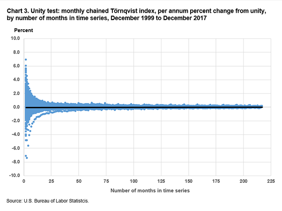
Charts 2–5 show the results of this iterative, sequentially run unity test when we used bounded Laspeyres and bounded Törnqvist formulas. Charts 2 and 3 show the per annum percent change in the monthly chained index value from unity (the beginning month in which the index equals 100) to the ending month in each iteration, up to the terminal month of December 2017. Chart 2 displays the results when the Laspeyres formula is used.
Chart 3 displays the results when the Törnqvist formula is used.
Charts 4 and 5 show the cumulative percent change in the monthly chained index value from unity (the beginning month in which the index equals 100) to the ending month in each iteration, up to the terminal month of December 2017. Chart 4 displays the results when the Laspeyres formula is used.
Chart 5 displays the results when the Törnqvist formula is used.
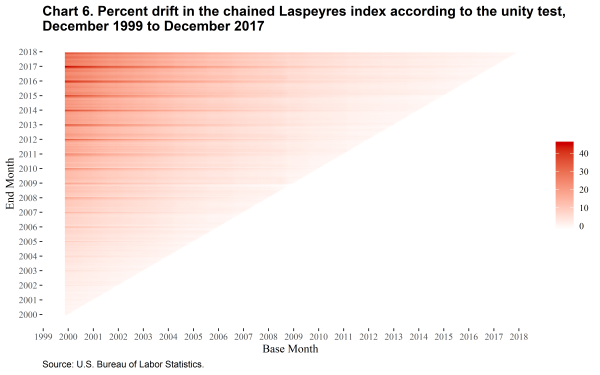
Chart 6 shows the accumulated amount of drift in the Laspeyres index between each pair of base and end months in the form of a heatmap.
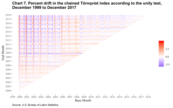
Chart 7 shows the accumulated amount of drift in the chained Törnqvist index.
The chained Laspeyres index shows substantial upward drift in almost all periods, while the chained Törnqvist index shows a seasonal pattern with strong upward drift when December is the base month and slight downward drift for most of the rest of the year. Several months also stand out as having stronger effects on drift, especially when December 1999 is the base month and the end months are in late 2008.
In these charts, we observe chain drift when the Laspeyres formula is used (charts 2 and 4) but not when the Törnqvist formula is used (charts 3 and 5). Table 1 shows summary statistics for the per annum percent changes from unity for the Laspeyres and Törnqvist formulas.
Table 1. Summary statistics for the per annum percent changes from unity for the Laspeyres and Törnqvist formulas, 1999–2017 | Statistic | Laspeyres | Törnqvist |
|---|
Mean | 1.00 | 0.05 |
|---|
Median | 1.00 | 0.00 |
|---|
Standard deviation | 0.43 | 0.37 |
|---|
Table 2 shows the percentage of months in the time series in which we observe upward or downward annual drift (on a cumulative basis).
Table 2. Percentage of months in which upward or downward per annum drift was observed, 1999–2017 | Drift | Laspeyres | Törnqvist |
|---|
Upward | 99.0 | 50.4 |
|---|
Downward | 1.0 | 49.6 |
|---|
From the preceding charts and tables, we conclude that chain drift in a monthly chained Törnqvist index at the U.S. city average, all-items level, is minimal, compared with the drift in a monthly chained Laspeyres index at the same level, which is sizeable.
Circularity test
We conducted a circularity test by comparing chained and direct versions of the CPI-U, U.S. city average, all-items index, using both a Laspeyres formula and a Törnqvist formula. The relevant comparisons are between the chained and direct Laspeyres index and between the chained and direct Törnqvist index. In both cases, we observed visible drift. The CPI-U, U.S. city average, all-items index calculated using a Laspeyres formula with monthly chaining exhibits upward drift relative to the same index directly calculated using a Laspeyres formula (without chaining). When the CPI-U, U.S. city average, all-items index is calculated using a Törnqvist formula with monthly chaining, it also exhibits upward drift relative to the same index directly calculated using a Törnqvist formula. The Törnqvist finding conflicts with a previous empirical analysis by Klick that showed lower drift for the chained CPI-U, U.S. city average, all-items index using a Törnqvist formula.39
The preceding analysis suggests that the existence and extent of chain drift may depend on the choice of base period. We investigated this issue by changing the base period to 2000 and conducting additional circularity tests. We set calendar year 2000 as the base period in the direct Törnqvist calculations. Chart 8 shows the results when we compared the direct Törnqvist index with the monthly chained version, the former rebased so that the average annual index in 2000 was equal to 100, and we observed no significant drift.
Chart 8. Circularity test for chained and direct Törnqvist indexes, with 12-month base, December 2000 to December 2017| Month and year | Chained Törnqvist index | Direct Törnqvist index |
|---|
Dec 2000 | 101.993 | 100.000 |
|---|
Jan 2001 | 101.262 | 101.446 |
|---|
Feb 2001 | 101.617 | 101.801 |
|---|
Mar 2001 | 101.870 | 102.004 |
|---|
Apr 2001 | 102.195 | 102.337 |
|---|
May 2001 | 102.547 | 102.639 |
|---|
Jun 2001 | 102.810 | 102.888 |
|---|
Jul 2001 | 102.484 | 102.510 |
|---|
Aug 2001 | 102.557 | 102.548 |
|---|
Sep 2001 | 102.898 | 102.915 |
|---|
Oct 2001 | 102.630 | 102.457 |
|---|
Nov 2001 | 102.396 | 102.188 |
|---|
Dec 2001 | 101.899 | 101.403 |
|---|
Jan 2002 | 102.135 | 102.269 |
|---|
Feb 2002 | 102.464 | 102.399 |
|---|
Mar 2002 | 103.040 | 102.988 |
|---|
Apr 2002 | 103.608 | 103.599 |
|---|
May 2002 | 103.587 | 103.528 |
|---|
Jun 2002 | 103.600 | 103.661 |
|---|
Jul 2002 | 103.708 | 103.693 |
|---|
Aug 2002 | 103.988 | 104.082 |
|---|
Sep 2002 | 104.193 | 104.318 |
|---|
Oct 2002 | 104.380 | 104.285 |
|---|
Nov 2002 | 104.345 | 104.205 |
|---|
Dec 2002 | 104.052 | 103.412 |
|---|
Jan 2003 | 104.438 | 104.762 |
|---|
Feb 2003 | 105.184 | 105.402 |
|---|
Mar 2003 | 105.886 | 106.032 |
|---|
Apr 2003 | 105.634 | 105.716 |
|---|
May 2003 | 105.512 | 105.430 |
|---|
Jun 2003 | 105.613 | 105.519 |
|---|
Jul 2003 | 105.698 | 105.626 |
|---|
Aug 2003 | 106.110 | 105.954 |
|---|
Sep 2003 | 106.420 | 106.247 |
|---|
Oct 2003 | 106.349 | 106.203 |
|---|
Nov 2003 | 106.003 | 105.590 |
|---|
Dec 2003 | 105.811 | 104.991 |
|---|
Jan 2004 | 106.374 | 106.782 |
|---|
Feb 2004 | 106.975 | 107.001 |
|---|
Mar 2004 | 107.646 | 107.671 |
|---|
Apr 2004 | 107.957 | 107.874 |
|---|
May 2004 | 108.508 | 108.104 |
|---|
Jun 2004 | 108.779 | 108.564 |
|---|
Jul 2004 | 108.622 | 108.265 |
|---|
Aug 2004 | 108.645 | 108.689 |
|---|
Sep 2004 | 108.928 | 108.661 |
|---|
Oct 2004 | 109.509 | 109.140 |
|---|
Nov 2004 | 109.577 | 109.092 |
|---|
Dec 2004 | 109.117 | 107.876 |
|---|
Jan 2005 | 109.261 | 109.701 |
|---|
Feb 2005 | 109.829 | 109.675 |
|---|
Mar 2005 | 110.562 | 110.359 |
|---|
Apr 2005 | 111.300 | 111.074 |
|---|
May 2005 | 111.255 | 111.093 |
|---|
Jun 2005 | 111.225 | 111.090 |
|---|
Jul 2005 | 111.623 | 111.283 |
|---|
Aug 2005 | 112.161 | 112.152 |
|---|
Sep 2005 | 113.417 | 113.224 |
|---|
Oct 2005 | 113.615 | 113.165 |
|---|
Nov 2005 | 112.801 | 112.365 |
|---|
Dec 2005 | 112.329 | 110.529 |
|---|
Jan 2006 | 113.063 | 113.890 |
|---|
Feb 2006 | 113.259 | 113.656 |
|---|
Mar 2006 | 113.865 | 114.069 |
|---|
Apr 2006 | 114.798 | 114.812 |
|---|
May 2006 | 115.335 | 115.055 |
|---|
Jun 2006 | 115.603 | 115.588 |
|---|
Jul 2006 | 115.904 | 115.847 |
|---|
Aug 2006 | 116.136 | 116.168 |
|---|
Sep 2006 | 115.660 | 115.683 |
|---|
Oct 2006 | 115.034 | 115.088 |
|---|
Nov 2006 | 114.818 | 114.281 |
|---|
Dec 2006 | 114.898 | 113.344 |
|---|
Jan 2007 | 115.158 | 115.892 |
|---|
Feb 2007 | 115.699 | 116.159 |
|---|
Mar 2007 | 116.746 | 116.768 |
|---|
Apr 2007 | 117.504 | 117.811 |
|---|
May 2007 | 118.131 | 117.847 |
|---|
Jun 2007 | 118.292 | 117.865 |
|---|
Jul 2007 | 118.197 | 117.916 |
|---|
Aug 2007 | 118.053 | 118.139 |
|---|
Sep 2007 | 118.423 | 118.646 |
|---|
Oct 2007 | 118.692 | 118.616 |
|---|
Nov 2007 | 119.305 | 118.108 |
|---|
Dec 2007 | 119.094 | 117.680 |
|---|
Jan 2008 | 119.617 | 120.749 |
|---|
Feb 2008 | 119.985 | 120.931 |
|---|
Mar 2008 | 121.084 | 121.956 |
|---|
Apr 2008 | 121.871 | 122.356 |
|---|
May 2008 | 122.907 | 122.921 |
|---|
Jun 2008 | 124.018 | 124.058 |
|---|
Jul 2008 | 124.582 | 124.941 |
|---|
Aug 2008 | 124.268 | 124.308 |
|---|
Sep 2008 | 124.259 | 123.850 |
|---|
Oct 2008 | 123.233 | 122.853 |
|---|
Nov 2008 | 120.863 | 120.019 |
|---|
Dec 2008 | 119.377 | 117.780 |
|---|
Jan 2009 | 119.839 | 121.298 |
|---|
Feb 2009 | 120.351 | 120.832 |
|---|
Mar 2009 | 120.578 | 120.897 |
|---|
Apr 2009 | 120.841 | 120.611 |
|---|
May 2009 | 121.212 | 121.308 |
|---|
Jun 2009 | 122.269 | 122.363 |
|---|
Jul 2009 | 122.059 | 122.277 |
|---|
Aug 2009 | 122.335 | 122.871 |
|---|
Sep 2009 | 122.459 | 122.938 |
|---|
Oct 2009 | 122.549 | 122.756 |
|---|
Nov 2009 | 122.583 | 121.379 |
|---|
Dec 2009 | 122.319 | 120.834 |
|---|
Jan 2010 | 122.738 | 124.587 |
|---|
Feb 2010 | 122.755 | 123.221 |
|---|
Mar 2010 | 123.245 | 123.258 |
|---|
Apr 2010 | 123.439 | 123.359 |
|---|
May 2010 | 123.511 | 124.105 |
|---|
Jun 2010 | 123.414 | 123.531 |
|---|
Jul 2010 | 123.404 | 123.739 |
|---|
Aug 2010 | 123.546 | 124.435 |
|---|
Sep 2010 | 123.649 | 124.077 |
|---|
Oct 2010 | 123.773 | 123.056 |
|---|
Nov 2010 | 123.720 | 122.465 |
|---|
Dec 2010 | 123.899 | 122.839 |
|---|
Jan 2011 | 124.501 | 126.167 |
|---|
Feb 2011 | 125.097 | 125.701 |
|---|
Mar 2011 | 126.321 | 126.756 |
|---|
Apr 2011 | 127.230 | 126.956 |
|---|
May 2011 | 127.773 | 128.059 |
|---|
Jun 2011 | 127.657 | 127.384 |
|---|
Jul 2011 | 127.766 | 128.649 |
|---|
Aug 2011 | 128.097 | 129.007 |
|---|
Sep 2011 | 128.357 | 129.319 |
|---|
Oct 2011 | 128.096 | 128.122 |
|---|
Nov 2011 | 127.894 | 126.754 |
|---|
Dec 2011 | 127.499 | 125.306 |
|---|
Jan 2012 | 128.089 | 130.304 |
|---|
Feb 2012 | 128.621 | 129.321 |
|---|
Mar 2012 | 129.605 | 129.443 |
|---|
Apr 2012 | 129.995 | 128.993 |
|---|
May 2012 | 129.869 | 129.914 |
|---|
Jun 2012 | 129.728 | 130.025 |
|---|
Jul 2012 | 129.459 | 130.104 |
|---|
Aug 2012 | 130.124 | 131.503 |
|---|
Sep 2012 | 130.690 | 131.383 |
|---|
Oct 2012 | 130.609 | 130.654 |
|---|
Nov 2012 | 129.976 | 128.407 |
|---|
Dec 2012 | 129.466 | 127.449 |
|---|
Jan 2013 | 129.852 | 131.476 |
|---|
Feb 2013 | 130.917 | 131.352 |
|---|
Mar 2013 | 131.299 | 131.451 |
|---|
Apr 2013 | 131.154 | 131.028 |
|---|
May 2013 | 131.346 | 131.455 |
|---|
Jun 2013 | 131.613 | 132.055 |
|---|
Jul 2013 | 131.633 | 132.065 |
|---|
Aug 2013 | 131.818 | 132.908 |
|---|
Sep 2013 | 131.980 | 132.229 |
|---|
Oct 2013 | 131.613 | 132.000 |
|---|
Nov 2013 | 131.332 | 130.546 |
|---|
Dec 2013 | 131.242 | 128.774 |
|---|
Jan 2014 | 131.750 | 133.618 |
|---|
Feb 2014 | 132.285 | 132.543 |
|---|
Mar 2014 | 133.128 | 133.741 |
|---|
Apr 2014 | 133.512 | 133.927 |
|---|
May 2014 | 133.983 | 133.723 |
|---|
Jun 2014 | 134.207 | 134.847 |
|---|
Jul 2014 | 134.165 | 134.443 |
|---|
Aug 2014 | 133.887 | 134.738 |
|---|
Sep 2014 | 133.939 | 134.927 |
|---|
Oct 2014 | 133.606 | 133.672 |
|---|
Nov 2014 | 132.803 | 130.971 |
|---|
Dec 2014 | 131.904 | 130.308 |
|---|
Jan 2015 | 131.210 | 132.310 |
|---|
Feb 2015 | 131.779 | 132.269 |
|---|
Mar 2015 | 132.697 | 133.012 |
|---|
Apr 2015 | 132.933 | 132.648 |
|---|
May 2015 | 133.689 | 133.610 |
|---|
Jun 2015 | 134.104 | 133.706 |
|---|
Jul 2015 | 134.097 | 134.070 |
|---|
Aug 2015 | 133.857 | 134.322 |
|---|
Sep 2015 | 133.565 | 134.363 |
|---|
Oct 2015 | 133.451 | 133.108 |
|---|
Nov 2015 | 133.084 | 131.383 |
|---|
Dec 2015 | 132.465 | 130.113 |
|---|
Jan 2016 | 132.653 | 134.130 |
|---|
Feb 2016 | 132.671 | 133.022 |
|---|
Mar 2016 | 133.378 | 133.243 |
|---|
Apr 2016 | 134.055 | 133.884 |
|---|
May 2016 | 134.611 | 134.619 |
|---|
Jun 2016 | 135.048 | 135.798 |
|---|
Jul 2016 | 134.731 | 134.969 |
|---|
Aug 2016 | 134.729 | 135.358 |
|---|
Sep 2016 | 135.032 | 135.795 |
|---|
Oct 2016 | 135.208 | 135.686 |
|---|
Nov 2016 | 134.869 | 132.516 |
|---|
Dec 2016 | 134.795 | 133.165 |
|---|
Jan 2017 | 135.640 | 137.063 |
|---|
Feb 2017 | 136.024 | 137.025 |
|---|
Mar 2017 | 136.105 | 136.311 |
|---|
Apr 2017 | 136.459 | 136.348 |
|---|
May 2017 | 136.592 | 137.009 |
|---|
Jun 2017 | 136.654 | 137.236 |
|---|
Jul 2017 | 136.426 | 136.067 |
|---|
Aug 2017 | 136.792 | 138.245 |
|---|
Sep 2017 | 137.523 | 138.711 |
|---|
Oct 2017 | 137.423 | 137.803 |
|---|
Nov 2017 | 137.349 | 136.708 |
|---|
Dec 2017 | 137.175 | 135.109 |
|---|
Törnqvist indexes with quarterly and annual chaining behave similarly to a chained index with a 12-month base. (See chart 9.) This implies that most of the drift we see in the monthly chained Törnqvist index is due to the base period rather than the effects of chaining in intermediate periods.
Chart 9. Chained Törnqvist indexes, by frequency, December 2000 to December 2017| Month and year | Monthly | Quarterly | Annual |
|---|
Dec 2000 | 102.0 | 102.0 | 102.0 |
|---|
Jan 2001 | 101.3 | 101.7 | 102.3 |
|---|
Feb 2001 | 101.6 | 101.7 | 102.3 |
|---|
Mar 2001 | 101.9 | 101.7 | 102.3 |
|---|
Apr 2001 | 102.2 | 102.6 | 102.3 |
|---|
May 2001 | 102.5 | 102.6 | 102.3 |
|---|
Jun 2001 | 102.8 | 102.6 | 102.3 |
|---|
Jul 2001 | 102.5 | 102.7 | 102.3 |
|---|
Aug 2001 | 102.6 | 102.7 | 102.3 |
|---|
Sep 2001 | 102.9 | 102.7 | 102.3 |
|---|
Oct 2001 | 102.6 | 102.3 | 102.3 |
|---|
Nov 2001 | 102.4 | 102.3 | 102.3 |
|---|
Dec 2001 | 101.9 | 102.3 | 102.3 |
|---|
Jan 2002 | 102.1 | 102.6 | 103.6 |
|---|
Feb 2002 | 102.5 | 102.6 | 103.6 |
|---|
Mar 2002 | 103.0 | 102.6 | 103.6 |
|---|
Apr 2002 | 103.6 | 103.7 | 103.6 |
|---|
May 2002 | 103.6 | 103.7 | 103.6 |
|---|
Jun 2002 | 103.6 | 103.7 | 103.6 |
|---|
Jul 2002 | 103.7 | 104.0 | 103.6 |
|---|
Aug 2002 | 104.0 | 104.0 | 103.6 |
|---|
Sep 2002 | 104.2 | 104.0 | 103.6 |
|---|
Oct 2002 | 104.4 | 104.3 | 103.6 |
|---|
Nov 2002 | 104.3 | 104.3 | 103.6 |
|---|
Dec 2002 | 104.1 | 104.3 | 103.6 |
|---|
Jan 2003 | 104.4 | 105.3 | 105.8 |
|---|
Feb 2003 | 105.2 | 105.3 | 105.8 |
|---|
Mar 2003 | 105.9 | 105.3 | 105.8 |
|---|
Apr 2003 | 105.6 | 105.7 | 105.8 |
|---|
May 2003 | 105.5 | 105.7 | 105.8 |
|---|
Jun 2003 | 105.6 | 105.7 | 105.8 |
|---|
Jul 2003 | 105.7 | 106.1 | 105.8 |
|---|
Aug 2003 | 106.1 | 106.1 | 105.8 |
|---|
Sep 2003 | 106.4 | 106.1 | 105.8 |
|---|
Oct 2003 | 106.3 | 106.1 | 105.8 |
|---|
Nov 2003 | 106.0 | 106.1 | 105.8 |
|---|
Dec 2003 | 105.8 | 106.1 | 105.8 |
|---|
Jan 2004 | 106.4 | 107.1 | 108.3 |
|---|
Feb 2004 | 107.0 | 107.1 | 108.3 |
|---|
Mar 2004 | 107.6 | 107.1 | 108.3 |
|---|
Apr 2004 | 108.0 | 108.5 | 108.3 |
|---|
May 2004 | 108.5 | 108.5 | 108.3 |
|---|
Jun 2004 | 108.8 | 108.5 | 108.3 |
|---|
Jul 2004 | 108.6 | 108.8 | 108.3 |
|---|
Aug 2004 | 108.6 | 108.8 | 108.3 |
|---|
Sep 2004 | 108.9 | 108.8 | 108.3 |
|---|
Oct 2004 | 109.5 | 109.5 | 108.3 |
|---|
Nov 2004 | 109.6 | 109.5 | 108.3 |
|---|
Dec 2004 | 109.1 | 109.5 | 108.3 |
|---|
Jan 2005 | 109.3 | 110.1 | 111.7 |
|---|
Feb 2005 | 109.8 | 110.1 | 111.7 |
|---|
Mar 2005 | 110.6 | 110.1 | 111.7 |
|---|
Apr 2005 | 111.3 | 111.5 | 111.7 |
|---|
May 2005 | 111.3 | 111.5 | 111.7 |
|---|
Jun 2005 | 111.2 | 111.5 | 111.7 |
|---|
Jul 2005 | 111.6 | 112.6 | 111.7 |
|---|
Aug 2005 | 112.2 | 112.6 | 111.7 |
|---|
Sep 2005 | 113.4 | 112.6 | 111.7 |
|---|
Oct 2005 | 113.6 | 113.1 | 111.7 |
|---|
Nov 2005 | 112.8 | 113.1 | 111.7 |
|---|
Dec 2005 | 112.3 | 113.1 | 111.7 |
|---|
Jan 2006 | 113.1 | 113.7 | 115.1 |
|---|
Feb 2006 | 113.3 | 113.7 | 115.1 |
|---|
Mar 2006 | 113.9 | 113.7 | 115.1 |
|---|
Apr 2006 | 114.8 | 115.6 | 115.1 |
|---|
May 2006 | 115.3 | 115.6 | 115.1 |
|---|
Jun 2006 | 115.6 | 115.6 | 115.1 |
|---|
Jul 2006 | 115.9 | 116.2 | 115.1 |
|---|
Aug 2006 | 116.1 | 116.2 | 115.1 |
|---|
Sep 2006 | 115.7 | 116.2 | 115.1 |
|---|
Oct 2006 | 115.0 | 115.2 | 115.1 |
|---|
Nov 2006 | 114.8 | 115.2 | 115.1 |
|---|
Dec 2006 | 114.9 | 115.2 | 115.1 |
|---|
Jan 2007 | 115.2 | 116.3 | 118.1 |
|---|
Feb 2007 | 115.7 | 116.3 | 118.1 |
|---|
Mar 2007 | 116.7 | 116.3 | 118.1 |
|---|
Apr 2007 | 117.5 | 118.3 | 118.1 |
|---|
May 2007 | 118.1 | 118.3 | 118.1 |
|---|
Jun 2007 | 118.3 | 118.3 | 118.1 |
|---|
Jul 2007 | 118.2 | 118.6 | 118.1 |
|---|
Aug 2007 | 118.1 | 118.6 | 118.1 |
|---|
Sep 2007 | 118.4 | 118.6 | 118.1 |
|---|
Oct 2007 | 118.7 | 119.4 | 118.1 |
|---|
Nov 2007 | 119.3 | 119.4 | 118.1 |
|---|
Dec 2007 | 119.1 | 119.4 | 118.1 |
|---|
Jan 2008 | 119.6 | 120.7 | 122.4 |
|---|
Feb 2008 | 120.0 | 120.7 | 122.4 |
|---|
Mar 2008 | 121.1 | 120.7 | 122.4 |
|---|
Apr 2008 | 121.9 | 123.3 | 122.4 |
|---|
May 2008 | 122.9 | 123.3 | 122.4 |
|---|
Jun 2008 | 124.0 | 123.3 | 122.4 |
|---|
Jul 2008 | 124.6 | 124.7 | 122.4 |
|---|
Aug 2008 | 124.3 | 124.7 | 122.4 |
|---|
Sep 2008 | 124.3 | 124.7 | 122.4 |
|---|
Oct 2008 | 123.2 | 121.4 | 122.4 |
|---|
Nov 2008 | 120.9 | 121.4 | 122.4 |
|---|
Dec 2008 | 119.4 | 121.4 | 122.4 |
|---|
Jan 2009 | 119.8 | 120.5 | 121.6 |
|---|
Feb 2009 | 120.4 | 120.5 | 121.6 |
|---|
Mar 2009 | 120.6 | 120.5 | 121.6 |
|---|
Apr 2009 | 120.8 | 121.7 | 121.6 |
|---|
May 2009 | 121.2 | 121.7 | 121.6 |
|---|
Jun 2009 | 122.3 | 121.7 | 121.6 |
|---|
Jul 2009 | 122.1 | 122.5 | 121.6 |
|---|
Aug 2009 | 122.3 | 122.5 | 121.6 |
|---|
Sep 2009 | 122.5 | 122.5 | 121.6 |
|---|
Oct 2009 | 122.5 | 122.7 | 121.6 |
|---|
Nov 2009 | 122.6 | 122.7 | 121.6 |
|---|
Dec 2009 | 122.3 | 122.7 | 121.6 |
|---|
Jan 2010 | 122.7 | 123.1 | 123.4 |
|---|
Feb 2010 | 122.8 | 123.1 | 123.4 |
|---|
Mar 2010 | 123.2 | 123.1 | 123.4 |
|---|
Apr 2010 | 123.4 | 123.7 | 123.4 |
|---|
May 2010 | 123.5 | 123.7 | 123.4 |
|---|
Jun 2010 | 123.4 | 123.7 | 123.4 |
|---|
Jul 2010 | 123.4 | 123.8 | 123.4 |
|---|
Aug 2010 | 123.5 | 123.8 | 123.4 |
|---|
Sep 2010 | 123.6 | 123.8 | 123.4 |
|---|
Oct 2010 | 123.8 | 124.0 | 123.4 |
|---|
Nov 2010 | 123.7 | 124.0 | 123.4 |
|---|
Dec 2010 | 123.9 | 124.0 | 123.4 |
|---|
Jan 2011 | 124.5 | 125.6 | 127.1 |
|---|
Feb 2011 | 125.1 | 125.6 | 127.1 |
|---|
Mar 2011 | 126.3 | 125.6 | 127.1 |
|---|
Apr 2011 | 127.2 | 127.8 | 127.1 |
|---|
May 2011 | 127.8 | 127.8 | 127.1 |
|---|
Jun 2011 | 127.7 | 127.8 | 127.1 |
|---|
Jul 2011 | 127.8 | 128.3 | 127.1 |
|---|
Aug 2011 | 128.1 | 128.3 | 127.1 |
|---|
Sep 2011 | 128.4 | 128.3 | 127.1 |
|---|
Oct 2011 | 128.1 | 128.0 | 127.1 |
|---|
Nov 2011 | 127.9 | 128.0 | 127.1 |
|---|
Dec 2011 | 127.5 | 128.0 | 127.1 |
|---|
Jan 2012 | 128.1 | 129.0 | 129.6 |
|---|
Feb 2012 | 128.6 | 129.0 | 129.6 |
|---|
Mar 2012 | 129.6 | 129.0 | 129.6 |
|---|
Apr 2012 | 130.0 | 130.1 | 129.6 |
|---|
May 2012 | 129.9 | 130.1 | 129.6 |
|---|
Jun 2012 | 129.7 | 130.1 | 129.6 |
|---|
Jul 2012 | 129.5 | 130.3 | 129.6 |
|---|
Aug 2012 | 130.1 | 130.3 | 129.6 |
|---|
Sep 2012 | 130.7 | 130.3 | 129.6 |
|---|
Oct 2012 | 130.6 | 130.3 | 129.6 |
|---|
Nov 2012 | 130.0 | 130.3 | 129.6 |
|---|
Dec 2012 | 129.5 | 130.3 | 129.6 |
|---|
Jan 2013 | 129.9 | 131.0 | 131.3 |
|---|
Feb 2013 | 130.9 | 131.0 | 131.3 |
|---|
Mar 2013 | 131.3 | 131.0 | 131.3 |
|---|
Apr 2013 | 131.2 | 131.7 | 131.3 |
|---|
May 2013 | 131.3 | 131.7 | 131.3 |
|---|
Jun 2013 | 131.6 | 131.7 | 131.3 |
|---|
Jul 2013 | 131.6 | 132.1 | 131.3 |
|---|
Aug 2013 | 131.8 | 132.1 | 131.3 |
|---|
Sep 2013 | 132.0 | 132.1 | 131.3 |
|---|
Oct 2013 | 131.6 | 131.7 | 131.3 |
|---|
Nov 2013 | 131.3 | 131.7 | 131.3 |
|---|
Dec 2013 | 131.2 | 131.7 | 131.3 |
|---|
Jan 2014 | 131.7 | 132.7 | 133.2 |
|---|
Feb 2014 | 132.3 | 132.7 | 133.2 |
|---|
Mar 2014 | 133.1 | 132.7 | 133.2 |
|---|
Apr 2014 | 133.5 | 134.2 | 133.2 |
|---|
May 2014 | 134.0 | 134.2 | 133.2 |
|---|
Jun 2014 | 134.2 | 134.2 | 133.2 |
|---|
Jul 2014 | 134.2 | 134.4 | 133.2 |
|---|
Aug 2014 | 133.9 | 134.4 | 133.2 |
|---|
Sep 2014 | 133.9 | 134.4 | 133.2 |
|---|
Oct 2014 | 133.6 | 133.2 | 133.2 |
|---|
Nov 2014 | 132.8 | 133.2 | 133.2 |
|---|
Dec 2014 | 131.9 | 133.2 | 133.2 |
|---|
Jan 2015 | 131.2 | 132.3 | 133.1 |
|---|
Feb 2015 | 131.8 | 132.3 | 133.1 |
|---|
Mar 2015 | 132.7 | 132.3 | 133.1 |
|---|
Apr 2015 | 132.9 | 134.0 | 133.1 |
|---|
May 2015 | 133.7 | 134.0 | 133.1 |
|---|
Jun 2015 | 134.1 | 134.0 | 133.1 |
|---|
Jul 2015 | 134.1 | 134.3 | 133.1 |
|---|
Aug 2015 | 133.9 | 134.3 | 133.1 |
|---|
Sep 2015 | 133.6 | 134.3 | 133.1 |
|---|
Oct 2015 | 133.5 | 133.5 | 133.1 |
|---|
Nov 2015 | 133.1 | 133.5 | 133.1 |
|---|
Dec 2015 | 132.5 | 133.5 | 133.1 |
|---|
Jan 2016 | 132.7 | 133.4 | 134.5 |
|---|
Feb 2016 | 132.7 | 133.4 | 134.5 |
|---|
Mar 2016 | 133.4 | 133.4 | 134.5 |
|---|
Apr 2016 | 134.1 | 135.1 | 134.5 |
|---|
May 2016 | 134.6 | 135.1 | 134.5 |
|---|
Jun 2016 | 135.0 | 135.1 | 134.5 |
|---|
Jul 2016 | 134.7 | 135.5 | 134.5 |
|---|
Aug 2016 | 134.7 | 135.5 | 134.5 |
|---|
Sep 2016 | 135.0 | 135.5 | 134.5 |
|---|
Oct 2016 | 135.2 | 135.6 | 134.5 |
|---|
Nov 2016 | 134.9 | 135.6 | 134.5 |
|---|
Dec 2016 | 134.8 | 135.6 | 134.5 |
|---|
Jan 2017 | 135.6 | 136.7 | 137.1 |
|---|
Feb 2017 | 136.0 | 136.7 | 137.1 |
|---|
Mar 2017 | 136.1 | 136.7 | 137.1 |
|---|
Apr 2017 | 136.5 | 137.3 | 137.1 |
|---|
May 2017 | 136.6 | 137.3 | 137.1 |
|---|
Jun 2017 | 136.7 | 137.3 | 137.1 |
|---|
Jul 2017 | 136.4 | 137.7 | 137.1 |
|---|
Aug 2017 | 136.8 | 137.7 | 137.1 |
|---|
Sep 2017 | 137.5 | 137.7 | 137.1 |
|---|
Oct 2017 | 137.4 | 138.1 | 137.1 |
|---|
Nov 2017 | 137.3 | 138.1 | 137.1 |
|---|
Dec 2017 | 137.2 | 138.1 | 137.1 |
|---|
Multilateral index comparisons
The CCDI index provides an alternative measure of price change. In general, a multilateral chained index is more representative than a direct index while maintaining transitivity and thereby avoiding chain drift. The CCDI index also avoids the base-period sensitivity issue. We used the IndexNumR package in R to test various versions of the CCDI index by varying the method of splicing and changing window length.40
Chart 10 displays the chained and direct Törnqvist indexes discussed previously compared with a full-period CCDI index and the results of applying various extension methods to extend a CCDI index.
Chart 10. Törnqvist index method compared with various CCDI methods, December 1999 to December 2017 (1999 = 100)| Month and year | Chained Törnqvist | Direct Törnqvist | CCDI | Mean, 13 months | Window splice, 13 months | Movement, 13 months | Mean, 24 months | Window splice, 24 months | Movement, 24 months | Mean, 36 months | Window splice, 36 months | Movement, 36 months |
|---|
Dec 1999 | 100.000 | 100.000 | 100.000 | 100.000 | 100.000 | 100.000 | 100.000 | 100.000 | 100.000 | 100.000 | 100.000 | 100.000 |
|---|
Jan 2000 | 100.302 | 100.302 | 97.628 | 100.154 | 100.154 | 100.154 | 100.005 | 100.005 | 100.005 | 99.835 | 99.835 | 99.835 |
|---|
Feb 2000 | 100.828 | 100.804 | 98.744 | 100.679 | 100.679 | 100.679 | 100.558 | 100.558 | 100.558 | 100.421 | 100.421 | 100.421 |
|---|
Mar 2000 | 101.601 | 101.532 | 99.930 | 101.488 | 101.488 | 101.488 | 101.398 | 101.398 | 101.398 | 101.270 | 101.270 | 101.270 |
|---|
Apr 2000 | 101.663 | 101.599 | 100.084 | 101.573 | 101.573 | 101.573 | 101.498 | 101.498 | 101.498 | 101.370 | 101.370 | 101.370 |
|---|
May 2000 | 101.687 | 101.608 | 100.519 | 101.633 | 101.633 | 101.633 | 101.596 | 101.596 | 101.596 | 101.497 | 101.497 | 101.497 |
|---|
Jun 2000 | 102.105 | 102.026 | 100.495 | 102.054 | 102.054 | 102.054 | 102.001 | 102.001 | 102.001 | 101.874 | 101.874 | 101.874 |
|---|
Jul 2000 | 102.281 | 102.226 | 100.642 | 102.246 | 102.246 | 102.246 | 102.211 | 102.211 | 102.211 | 102.081 | 102.081 | 102.081 |
|---|
Aug 2000 | 102.282 | 102.236 | 100.188 | 102.243 | 102.243 | 102.243 | 102.193 | 102.193 | 102.193 | 102.045 | 102.045 | 102.045 |
|---|
Sep 2000 | 102.771 | 102.706 | 100.511 | 102.731 | 102.731 | 102.731 | 102.663 | 102.663 | 102.663 | 102.490 | 102.490 | 102.490 |
|---|
Oct 2000 | 102.894 | 102.851 | 100.876 | 102.857 | 102.857 | 102.857 | 102.791 | 102.791 | 102.791 | 102.633 | 102.633 | 102.633 |
|---|
Nov 2000 | 102.861 | 102.751 | 101.665 | 102.822 | 102.822 | 102.822 | 102.801 | 102.801 | 102.801 | 102.705 | 102.705 | 102.705 |
|---|
Dec 2000 | 102.637 | 102.429 | 102.644 | 102.599 | 102.599 | 102.599 | 102.654 | 102.654 | 102.654 | 102.663 | 102.663 | 102.663 |
|---|
Jan 2001 | 103.280 | 103.509 | 100.549 | 103.477 | 103.507 | 103.446 | 103.343 | 103.343 | 103.343 | 103.146 | 103.146 | 103.146 |
|---|
Feb 2001 | 103.642 | 103.844 | 101.653 | 103.823 | 103.866 | 103.808 | 103.742 | 103.742 | 103.742 | 103.597 | 103.597 | 103.597 |
|---|
Mar 2001 | 103.900 | 103.979 | 102.274 | 104.036 | 104.081 | 104.038 | 103.992 | 103.992 | 103.992 | 103.875 | 103.875 | 103.875 |
|---|
Apr 2001 | 104.231 | 104.344 | 102.309 | 104.372 | 104.418 | 104.379 | 104.314 | 104.314 | 104.314 | 104.159 | 104.159 | 104.159 |
|---|
May 2001 | 104.590 | 104.540 | 102.851 | 104.697 | 104.734 | 104.711 | 104.627 | 104.627 | 104.627 | 104.468 | 104.468 | 104.468 |
|---|
Jun 2001 | 104.859 | 104.764 | 103.031 | 104.964 | 105.001 | 104.975 | 104.884 | 104.884 | 104.884 | 104.717 | 104.717 | 104.717 |
|---|
Jul 2001 | 104.526 | 104.419 | 102.604 | 104.596 | 104.625 | 104.609 | 104.521 | 104.521 | 104.521 | 104.372 | 104.372 | 104.372 |
|---|
Aug 2001 | 104.601 | 104.424 | 102.247 | 104.642 | 104.673 | 104.653 | 104.556 | 104.556 | 104.556 | 104.386 | 104.386 | 104.386 |
|---|
Sep 2001 | 104.948 | 104.747 | 102.741 | 104.965 | 105.005 | 104.978 | 104.893 | 104.893 | 104.893 | 104.708 | 104.708 | 104.708 |
|---|
Oct 2001 | 104.675 | 104.256 | 103.024 | 104.544 | 104.586 | 104.574 | 104.463 | 104.463 | 104.463 | 104.345 | 104.345 | 104.345 |
|---|
Nov 2001 | 104.436 | 103.970 | 103.011 | 104.270 | 104.302 | 104.306 | 104.195 | 104.195 | 104.195 | 104.099 | 104.099 | 104.099 |
|---|
Dec 2001 | 103.930 | 103.002 | 103.456 | 103.674 | 103.667 | 103.713 | 103.511 | 103.520 | 103.509 | 103.506 | 103.506 | 103.506 |
|---|
Jan 2002 | 104.170 | 104.087 | 101.409 | 104.177 | 104.191 | 104.170 | 104.176 | 104.191 | 104.152 | 104.012 | 104.012 | 104.012 |
|---|
Feb 2002 | 104.506 | 104.160 | 102.484 | 104.425 | 104.425 | 104.430 | 104.370 | 104.384 | 104.359 | 104.249 | 104.249 | 104.249 |
|---|
Mar 2002 | 105.093 | 104.734 | 103.175 | 105.044 | 105.033 | 105.040 | 104.977 | 104.992 | 104.968 | 104.857 | 104.857 | 104.857 |
|---|
Apr 2002 | 105.673 | 105.313 | 103.950 | 105.665 | 105.660 | 105.652 | 105.600 | 105.611 | 105.592 | 105.470 | 105.470 | 105.470 |
|---|
May 2002 | 105.651 | 105.152 | 103.962 | 105.623 | 105.626 | 105.613 | 105.560 | 105.572 | 105.552 | 105.423 | 105.423 | 105.423 |
|---|
Jun 2002 | 105.664 | 105.271 | 103.793 | 105.689 | 105.701 | 105.678 | 105.658 | 105.670 | 105.646 | 105.519 | 105.519 | 105.519 |
|---|
Jul 2002 | 105.775 | 105.233 | 104.001 | 105.781 | 105.797 | 105.777 | 105.740 | 105.755 | 105.732 | 105.595 | 105.595 | 105.595 |
|---|
Aug 2002 | 106.060 | 105.615 | 103.797 | 106.075 | 106.109 | 106.075 | 106.084 | 106.107 | 106.074 | 105.940 | 105.940 | 105.940 |
|---|
Sep 2002 | 106.269 | 105.864 | 104.158 | 106.288 | 106.334 | 106.298 | 106.290 | 106.319 | 106.287 | 106.163 | 106.163 | 106.163 |
|---|
Oct 2002 | 106.460 | 105.781 | 104.855 | 106.411 | 106.452 | 106.434 | 106.360 | 106.379 | 106.366 | 106.209 | 106.209 | 106.209 |
|---|
Nov 2002 | 106.424 | 105.674 | 104.984 | 106.395 | 106.430 | 106.414 | 106.318 | 106.313 | 106.323 | 106.153 | 106.153 | 106.153 |
|---|
Dec 2002 | 106.125 | 104.732 | 105.389 | 106.021 | 106.024 | 106.042 | 105.854 | 105.862 | 105.853 | 105.579 | 105.588 | 105.573 |
|---|
Jan 2003 | 106.519 | 106.253 | 104.139 | 106.693 | 106.724 | 106.672 | 106.672 | 106.681 | 106.650 | 106.577 | 106.590 | 106.550 |
|---|
Feb 2003 | 107.280 | 106.878 | 105.342 | 107.390 | 107.426 | 107.388 | 107.354 | 107.364 | 107.342 | 107.246 | 107.261 | 107.227 |
|---|
Mar 2003 | 107.996 | 107.525 | 106.043 | 108.057 | 108.096 | 108.065 | 108.028 | 108.049 | 108.022 | 107.913 | 107.929 | 107.899 |
|---|
Apr 2003 | 107.739 | 107.160 | 105.878 | 107.770 | 107.810 | 107.787 | 107.738 | 107.761 | 107.740 | 107.622 | 107.631 | 107.611 |
|---|
May 2003 | 107.614 | 106.812 | 105.843 | 107.604 | 107.642 | 107.626 | 107.557 | 107.584 | 107.561 | 107.421 | 107.430 | 107.410 |
|---|
Jun 2003 | 107.718 | 106.887 | 105.892 | 107.709 | 107.745 | 107.729 | 107.652 | 107.681 | 107.660 | 107.525 | 107.530 | 107.512 |
|---|
Jul 2003 | 107.804 | 107.021 | 105.864 | 107.811 | 107.841 | 107.829 | 107.757 | 107.793 | 107.767 | 107.639 | 107.645 | 107.623 |
|---|
Aug 2003 | 108.224 | 107.309 | 106.152 | 108.175 | 108.215 | 108.195 | 108.102 | 108.142 | 108.117 | 107.994 | 108.004 | 107.978 |
|---|
Sep 2003 | 108.541 | 107.593 | 106.589 | 108.435 | 108.472 | 108.462 | 108.360 | 108.393 | 108.378 | 108.255 | 108.265 | 108.242 |
|---|
Oct 2003 | 108.468 | 107.593 | 106.594 | 108.347 | 108.375 | 108.374 | 108.288 | 108.317 | 108.303 | 108.181 | 108.184 | 108.169 |
|---|
Nov 2003 | 108.115 | 106.950 | 106.416 | 107.973 | 107.992 | 107.996 | 107.879 | 107.889 | 107.895 | 107.716 | 107.697 | 107.706 |
|---|
Dec 2003 | 107.919 | 106.225 | 106.806 | 107.818 | 107.820 | 107.831 | 107.672 | 107.700 | 107.678 | 107.422 | 107.420 | 107.404 |
|---|
Jan 2004 | 108.494 | 108.226 | 106.321 | 108.592 | 108.625 | 108.580 | 108.607 | 108.638 | 108.600 | 108.540 | 108.542 | 108.506 |
|---|
Feb 2004 | 109.107 | 108.530 | 107.008 | 109.063 | 109.088 | 109.080 | 109.031 | 109.063 | 109.039 | 108.905 | 108.904 | 108.887 |
|---|
Mar 2004 | 109.791 | 109.108 | 107.762 | 109.731 | 109.759 | 109.748 | 109.703 | 109.735 | 109.714 | 109.593 | 109.599 | 109.575 |
|---|
Apr 2004 | 110.108 | 109.285 | 108.084 | 110.022 | 110.044 | 110.039 | 109.959 | 109.991 | 109.974 | 109.839 | 109.843 | 109.826 |
|---|
May 2004 | 110.670 | 109.395 | 108.806 | 110.520 | 110.536 | 110.538 | 110.393 | 110.422 | 110.412 | 110.228 | 110.233 | 110.218 |
|---|
Jun 2004 | 110.947 | 109.883 | 108.972 | 110.857 | 110.871 | 110.863 | 110.762 | 110.786 | 110.777 | 110.615 | 110.622 | 110.602 |
|---|
Jul 2004 | 110.786 | 109.551 | 108.768 | 110.691 | 110.705 | 110.695 | 110.611 | 110.643 | 110.622 | 110.453 | 110.468 | 110.443 |
|---|
Aug 2004 | 110.810 | 109.952 | 108.467 | 110.761 | 110.783 | 110.762 | 110.724 | 110.757 | 110.732 | 110.615 | 110.635 | 110.604 |
|---|
Sep 2004 | 111.099 | 109.886 | 108.981 | 110.977 | 110.994 | 110.984 | 110.879 | 110.902 | 110.897 | 110.732 | 110.746 | 110.731 |
|---|
Oct 2004 | 111.691 | 110.402 | 109.636 | 111.555 | 111.569 | 111.560 | 111.434 | 111.453 | 111.447 | 111.271 | 111.280 | 111.268 |
|---|
Nov 2004 | 111.760 | 110.286 | 109.965 | 111.609 | 111.610 | 111.610 | 111.494 | 111.499 | 111.505 | 111.315 | 111.306 | 111.309 |
|---|
Dec 2004 | 111.291 | 108.902 | 110.019 | 111.140 | 111.118 | 111.132 | 110.974 | 110.992 | 110.977 | 110.712 | 110.719 | 110.700 |
|---|
Jan 2005 | 111.438 | 110.965 | 109.256 | 111.547 | 111.542 | 111.503 | 111.526 | 111.547 | 111.513 | 111.466 | 111.476 | 111.436 |
|---|
Feb 2005 | 112.018 | 110.873 | 110.205 | 112.064 | 112.067 | 112.031 | 111.982 | 112.004 | 111.983 | 111.851 | 111.861 | 111.834 |
|---|
Mar 2005 | 112.765 | 111.526 | 110.907 | 112.823 | 112.825 | 112.790 | 112.723 | 112.741 | 112.723 | 112.566 | 112.575 | 112.553 |
|---|
Apr 2005 | 113.518 | 112.186 | 111.642 | 113.530 | 113.533 | 113.505 | 113.423 | 113.439 | 113.423 | 113.260 | 113.266 | 113.248 |
|---|
May 2005 | 113.472 | 112.247 | 111.487 | 113.496 | 113.497 | 113.470 | 113.399 | 113.412 | 113.394 | 113.229 | 113.236 | 113.215 |
|---|
Jun 2005 | 113.441 | 112.206 | 111.459 | 113.485 | 113.481 | 113.458 | 113.404 | 113.422 | 113.396 | 113.268 | 113.274 | 113.252 |
|---|
Jul 2005 | 113.847 | 112.339 | 111.895 | 113.855 | 113.850 | 113.828 | 113.763 | 113.784 | 113.760 | 113.618 | 113.631 | 113.604 |
|---|
Aug 2005 | 114.396 | 113.212 | 112.241 | 114.399 | 114.406 | 114.370 | 114.332 | 114.350 | 114.327 | 114.222 | 114.236 | 114.207 |
|---|
Sep 2005 | 115.677 | 114.258 | 113.555 | 115.661 | 115.662 | 115.638 | 115.554 | 115.569 | 115.551 | 115.393 | 115.399 | 115.386 |
|---|
Oct 2005 | 115.879 | 114.188 | 113.884 | 115.830 | 115.822 | 115.806 | 115.697 | 115.703 | 115.692 | 115.499 | 115.499 | 115.490 |
|---|
Nov 2005 | 115.049 | 113.395 | 113.251 | 115.090 | 115.072 | 115.053 | 114.986 | 114.979 | 114.968 | 114.792 | 114.777 | 114.774 |
|---|
Dec 2005 | 114.567 | 111.349 | 113.590 | 114.588 | 114.542 | 114.549 | 114.361 | 114.361 | 114.343 | 114.059 | 114.055 | 114.039 |
|---|
Jan 2006 | 115.316 | 114.961 | 113.541 | 115.682 | 115.669 | 115.598 | 115.663 | 115.678 | 115.617 | 115.571 | 115.572 | 115.526 |
|---|
Feb 2006 | 115.516 | 114.696 | 113.997 | 115.842 | 115.837 | 115.778 | 115.815 | 115.835 | 115.782 | 115.692 | 115.697 | 115.661 |
|---|
Mar 2006 | 116.134 | 115.079 | 114.604 | 116.458 | 116.456 | 116.406 | 116.411 | 116.437 | 116.388 | 116.274 | 116.278 | 116.246 |
|---|
Apr 2006 | 117.086 | 115.806 | 115.533 | 117.420 | 117.413 | 117.373 | 117.332 | 117.354 | 117.317 | 117.175 | 117.177 | 117.149 |
|---|
May 2006 | 117.633 | 115.967 | 116.004 | 117.955 | 117.949 | 117.908 | 117.823 | 117.839 | 117.808 | 117.622 | 117.620 | 117.596 |
|---|
Jun 2006 | 117.907 | 116.480 | 116.291 | 118.277 | 118.277 | 118.224 | 118.172 | 118.188 | 118.150 | 117.994 | 117.995 | 117.961 |
|---|
Jul 2006 | 118.214 | 116.697 | 116.513 | 118.550 | 118.554 | 118.505 | 118.435 | 118.460 | 118.414 | 118.248 | 118.249 | 118.218 |
|---|
Aug 2006 | 118.450 | 116.959 | 116.542 | 118.732 | 118.742 | 118.696 | 118.593 | 118.614 | 118.579 | 118.410 | 118.408 | 118.381 |
|---|
Sep 2006 | 117.965 | 116.552 | 116.074 | 118.183 | 118.201 | 118.156 | 118.071 | 118.090 | 118.055 | 117.901 | 117.899 | 117.871 |
|---|
Oct 2006 | 117.326 | 115.995 | 115.469 | 117.509 | 117.526 | 117.493 | 117.412 | 117.426 | 117.397 | 117.252 | 117.246 | 117.221 |
|---|
Nov 2006 | 117.106 | 115.125 | 115.464 | 117.236 | 117.247 | 117.228 | 117.107 | 117.106 | 117.096 | 116.910 | 116.889 | 116.881 |
|---|
Dec 2006 | 117.188 | 114.021 | 115.750 | 117.326 | 117.296 | 117.316 | 117.129 | 117.137 | 117.112 | 116.834 | 116.818 | 116.799 |
|---|
Jan 2007 | 117.453 | 116.672 | 115.713 | 117.811 | 117.796 | 117.766 | 117.729 | 117.737 | 117.694 | 117.601 | 117.591 | 117.545 |
|---|
Feb 2007 | 118.004 | 116.978 | 116.430 | 118.307 | 118.286 | 118.269 | 118.225 | 118.236 | 118.195 | 118.107 | 118.099 | 118.056 |
|---|
Mar 2007 | 119.072 | 117.537 | 117.505 | 119.396 | 119.373 | 119.355 | 119.281 | 119.293 | 119.257 | 119.109 | 119.103 | 119.065 |
|---|
Apr 2007 | 119.845 | 118.567 | 118.171 | 120.190 | 120.173 | 120.148 | 120.104 | 120.120 | 120.080 | 119.935 | 119.923 | 119.890 |
|---|
May 2007 | 120.485 | 118.492 | 118.680 | 120.771 | 120.756 | 120.738 | 120.676 | 120.695 | 120.657 | 120.468 | 120.454 | 120.425 |
|---|
Jun 2007 | 120.649 | 118.427 | 118.855 | 120.937 | 120.925 | 120.905 | 120.837 | 120.854 | 120.820 | 120.613 | 120.595 | 120.567 |
|---|
Jul 2007 | 120.552 | 118.506 | 118.876 | 120.869 | 120.863 | 120.839 | 120.787 | 120.810 | 120.768 | 120.584 | 120.572 | 120.532 |
|---|
Aug 2007 | 120.405 | 118.747 | 118.626 | 120.703 | 120.706 | 120.676 | 120.631 | 120.660 | 120.615 | 120.459 | 120.445 | 120.409 |
|---|
Sep 2007 | 120.783 | 119.295 | 119.044 | 121.082 | 121.088 | 121.057 | 120.995 | 121.023 | 120.986 | 120.837 | 120.822 | 120.787 |
|---|
Oct 2007 | 121.057 | 119.296 | 119.316 | 121.315 | 121.329 | 121.296 | 121.201 | 121.229 | 121.198 | 121.032 | 121.012 | 120.984 |
|---|
Nov 2007 | 121.682 | 118.640 | 120.019 | 121.900 | 121.899 | 121.889 | 121.725 | 121.717 | 121.729 | 121.464 | 121.420 | 121.420 |
|---|
Dec 2007 | 121.467 | 118.122 | 119.901 | 121.724 | 121.694 | 121.700 | 121.540 | 121.546 | 121.525 | 121.263 | 121.234 | 121.203 |
|---|
Jan 2008 | 122.008 | 121.394 | 120.500 | 122.462 | 122.452 | 122.409 | 122.403 | 122.413 | 122.373 | 122.277 | 122.250 | 122.202 |
|---|
Feb 2008 | 122.383 | 121.659 | 121.023 | 122.823 | 122.830 | 122.782 | 122.765 | 122.780 | 122.743 | 122.637 | 122.617 | 122.570 |
|---|
Mar 2008 | 123.503 | 122.691 | 122.004 | 123.877 | 123.885 | 123.857 | 123.832 | 123.851 | 123.820 | 123.696 | 123.678 | 123.638 |
|---|
Apr 2008 | 124.306 | 123.092 | 122.740 | 124.601 | 124.616 | 124.593 | 124.538 | 124.553 | 124.533 | 124.402 | 124.389 | 124.349 |
|---|
May 2008 | 125.363 | 123.601 | 123.623 | 125.558 | 125.561 | 125.561 | 125.474 | 125.488 | 125.471 | 125.314 | 125.306 | 125.269 |
|---|
Jun 2008 | 126.496 | 124.677 | 124.586 | 126.660 | 126.649 | 126.657 | 126.559 | 126.574 | 126.556 | 126.404 | 126.398 | 126.363 |
|---|
Jul 2008 | 127.072 | 125.602 | 125.266 | 127.331 | 127.310 | 127.311 | 127.254 | 127.261 | 127.245 | 127.122 | 127.120 | 127.080 |
|---|
Aug 2008 | 126.751 | 124.840 | 124.498 | 126.801 | 126.775 | 126.787 | 126.674 | 126.682 | 126.666 | 126.513 | 126.511 | 126.482 |
|---|
Sep 2008 | 126.742 | 124.390 | 124.409 | 126.713 | 126.684 | 126.695 | 126.557 | 126.566 | 126.551 | 126.366 | 126.360 | 126.340 |
|---|
Oct 2008 | 125.696 | 123.433 | 123.436 | 125.628 | 125.597 | 125.605 | 125.504 | 125.502 | 125.497 | 125.328 | 125.321 | 125.301 |
|---|
Nov 2008 | 123.278 | 120.606 | 121.148 | 122.921 | 122.885 | 122.914 | 122.829 | 122.812 | 122.828 | 122.625 | 122.593 | 122.607 |
|---|
Dec 2008 | 121.763 | 118.256 | 119.630 | 121.347 | 121.312 | 121.354 | 121.272 | 121.274 | 121.268 | 121.033 | 121.019 | 121.009 |
|---|
Jan 2009 | 122.233 | 121.965 | 120.509 | 122.013 | 122.003 | 122.006 | 122.077 | 122.086 | 122.067 | 122.007 | 121.993 | 121.970 |
|---|
Feb 2009 | 122.756 | 121.443 | 120.947 | 122.556 | 122.529 | 122.564 | 122.569 | 122.572 | 122.566 | 122.442 | 122.425 | 122.411 |
|---|
Mar 2009 | 122.988 | 121.516 | 121.146 | 122.794 | 122.759 | 122.790 | 122.780 | 122.783 | 122.779 | 122.663 | 122.644 | 122.631 |
|---|
Apr 2009 | 123.256 | 121.145 | 121.255 | 123.125 | 123.069 | 123.105 | 123.052 | 123.061 | 123.050 | 122.895 | 122.874 | 122.862 |
|---|
May 2009 | 123.634 | 121.786 | 121.802 | 123.647 | 123.606 | 123.599 | 123.591 | 123.606 | 123.587 | 123.454 | 123.435 | 123.416 |
|---|
Jun 2009 | 124.712 | 122.758 | 122.858 | 124.756 | 124.736 | 124.710 | 124.707 | 124.723 | 124.710 | 124.559 | 124.544 | 124.521 |
|---|
Jul 2009 | 124.498 | 122.668 | 122.599 | 124.499 | 124.484 | 124.471 | 124.460 | 124.484 | 124.465 | 124.328 | 124.321 | 124.292 |
|---|
Aug 2009 | 124.780 | 123.217 | 122.851 | 124.772 | 124.817 | 124.756 | 124.796 | 124.827 | 124.803 | 124.667 | 124.667 | 124.636 |
|---|
Sep 2009 | 124.906 | 123.324 | 123.006 | 124.803 | 124.868 | 124.820 | 124.815 | 124.848 | 124.831 | 124.695 | 124.701 | 124.672 |
|---|
Oct 2009 | 124.998 | 123.114 | 123.000 | 124.822 | 124.895 | 124.858 | 124.808 | 124.833 | 124.830 | 124.669 | 124.668 | 124.652 |
|---|
Nov 2009 | 125.033 | 121.600 | 122.899 | 124.786 | 124.840 | 124.829 | 124.749 | 124.763 | 124.775 | 124.545 | 124.524 | 124.531 |
|---|
Dec 2009 | 124.763 | 120.980 | 122.609 | 124.529 | 124.555 | 124.562 | 124.431 | 124.451 | 124.450 | 124.222 | 124.212 | 124.199 |
|---|
Jan 2010 | 125.191 | 124.908 | 123.567 | 125.148 | 125.181 | 125.152 | 125.156 | 125.178 | 125.164 | 125.089 | 125.082 | 125.053 |
|---|
Feb 2010 | 125.208 | 123.516 | 123.321 | 125.121 | 125.145 | 125.133 | 125.028 | 125.051 | 125.049 | 124.873 | 124.862 | 124.850 |
|---|
Mar 2010 | 125.709 | 123.523 | 123.711 | 125.625 | 125.651 | 125.636 | 125.568 | 125.587 | 125.585 | 125.394 | 125.383 | 125.370 |
|---|
Apr 2010 | 125.906 | 123.575 | 123.921 | 125.855 | 125.886 | 125.863 | 125.840 | 125.868 | 125.852 | 125.687 | 125.681 | 125.659 |
|---|
May 2010 | 125.979 | 124.301 | 124.150 | 125.875 | 125.900 | 125.890 | 125.887 | 125.930 | 125.901 | 125.783 | 125.780 | 125.757 |
|---|
Jun 2010 | 125.880 | 123.653 | 123.955 | 125.813 | 125.832 | 125.822 | 125.794 | 125.841 | 125.818 | 125.654 | 125.648 | 125.633 |
|---|
Jul 2010 | 125.870 | 123.856 | 124.008 | 125.820 | 125.845 | 125.822 | 125.819 | 125.889 | 125.850 | 125.679 | 125.679 | 125.656 |
|---|
Aug 2010 | 126.015 | 124.577 | 124.241 | 125.944 | 125.976 | 125.949 | 125.955 | 126.033 | 125.989 | 125.863 | 125.868 | 125.842 |
|---|
Sep 2010 | 126.121 | 124.195 | 124.257 | 126.037 | 126.074 | 126.043 | 126.040 | 126.122 | 126.082 | 125.953 | 125.960 | 125.936 |
|---|
Oct 2010 | 126.246 | 123.204 | 124.114 | 126.103 | 126.144 | 126.118 | 126.089 | 126.163 | 126.139 | 125.951 | 125.947 | 125.940 |
|---|
Nov 2010 | 126.192 | 122.513 | 123.988 | 126.021 | 126.048 | 126.039 | 125.979 | 126.043 | 126.028 | 125.803 | 125.787 | 125.790 |
|---|
Dec 2010 | 126.375 | 122.812 | 124.237 | 126.243 | 126.259 | 126.253 | 126.169 | 126.240 | 126.215 | 125.986 | 125.979 | 125.964 |
|---|
Jan 2011 | 126.989 | 126.324 | 125.452 | 126.946 | 126.973 | 126.939 | 126.968 | 127.038 | 127.008 | 126.849 | 126.842 | 126.821 |
|---|
Feb 2011 | 127.597 | 125.873 | 125.795 | 127.534 | 127.558 | 127.532 | 127.569 | 127.648 | 127.614 | 127.389 | 127.383 | 127.368 |
|---|
Mar 2011 | 128.846 | 126.834 | 126.916 | 128.765 | 128.786 | 128.766 | 128.745 | 128.831 | 128.802 | 128.604 | 128.599 | 128.583 |
|---|
Apr 2011 | 129.772 | 126.951 | 127.567 | 129.608 | 129.625 | 129.615 | 129.583 | 129.668 | 129.648 | 129.465 | 129.465 | 129.446 |
|---|
May 2011 | 130.326 | 128.054 | 128.240 | 130.102 | 130.115 | 130.112 | 130.050 | 130.131 | 130.121 | 129.939 | 129.951 | 129.924 |
|---|
Jun 2011 | 130.209 | 127.333 | 128.101 | 130.072 | 130.084 | 130.071 | 130.044 | 130.130 | 130.106 | 129.927 | 129.941 | 129.916 |
|---|
Jul 2011 | 130.319 | 128.718 | 128.492 | 130.206 | 130.223 | 130.201 | 130.191 | 130.280 | 130.253 | 130.090 | 130.120 | 130.083 |
|---|
Aug 2011 | 130.658 | 128.987 | 128.819 | 130.509 | 130.530 | 130.510 | 130.498 | 130.587 | 130.561 | 130.417 | 130.453 | 130.412 |
|---|
Sep 2011 | 130.923 | 129.293 | 128.968 | 130.688 | 130.711 | 130.697 | 130.664 | 130.753 | 130.730 | 130.550 | 130.587 | 130.555 |
|---|
Oct 2011 | 130.656 | 128.118 | 128.456 | 130.367 | 130.390 | 130.383 | 130.329 | 130.404 | 130.397 | 130.165 | 130.194 | 130.175 |
|---|
Nov 2011 | 130.451 | 126.664 | 128.008 | 130.144 | 130.153 | 130.159 | 130.070 | 130.137 | 130.133 | 129.882 | 129.902 | 129.890 |
|---|
Dec 2011 | 130.047 | 125.068 | 127.420 | 129.762 | 129.761 | 129.768 | 129.681 | 129.755 | 129.737 | 129.477 | 129.502 | 129.481 |
|---|
Jan 2012 | 130.648 | 130.272 | 129.143 | 130.529 | 130.538 | 130.515 | 130.559 | 130.635 | 130.602 | 130.491 | 130.516 | 130.482 |
|---|
Feb 2012 | 131.192 | 129.301 | 129.246 | 131.009 | 131.019 | 131.005 | 131.017 | 131.093 | 131.069 | 130.899 | 130.928 | 130.900 |
|---|
Mar 2012 | 132.195 | 129.319 | 129.997 | 132.014 | 132.026 | 132.007 | 131.984 | 132.058 | 132.039 | 131.831 | 131.863 | 131.838 |
|---|
Apr 2012 | 132.592 | 128.769 | 130.102 | 132.390 | 132.402 | 132.386 | 132.324 | 132.393 | 132.380 | 132.132 | 132.158 | 132.142 |
|---|
May 2012 | 132.464 | 129.679 | 130.311 | 132.292 | 132.304 | 132.283 | 132.247 | 132.318 | 132.298 | 132.090 | 132.114 | 132.095 |
|---|
Jun 2012 | 132.320 | 129.766 | 130.319 | 132.161 | 132.170 | 132.151 | 132.127 | 132.203 | 132.178 | 131.997 | 132.029 | 132.000 |
|---|
Jul 2012 | 132.047 | 129.854 | 130.200 | 131.911 | 131.926 | 131.900 | 131.895 | 131.978 | 131.947 | 131.793 | 131.834 | 131.798 |
|---|
Aug 2012 | 132.725 | 131.275 | 131.045 | 132.576 | 132.605 | 132.570 | 132.582 | 132.669 | 132.639 | 132.479 | 132.524 | 132.490 |
|---|
Sep 2012 | 133.302 | 131.110 | 131.372 | 133.106 | 133.145 | 133.110 | 133.096 | 133.183 | 133.159 | 132.960 | 133.007 | 132.978 |
|---|
Oct 2012 | 133.220 | 130.401 | 131.125 | 133.001 | 133.040 | 133.012 | 132.975 | 133.055 | 133.041 | 132.844 | 132.882 | 132.864 |
|---|
Nov 2012 | 132.573 | 128.061 | 130.032 | 132.375 | 132.398 | 132.386 | 132.305 | 132.375 | 132.369 | 132.109 | 132.138 | 132.130 |
|---|
Dec 2012 | 132.053 | 126.929 | 129.450 | 131.899 | 131.903 | 131.897 | 131.813 | 131.886 | 131.869 | 131.610 | 131.645 | 131.621 |
|---|
Jan 2013 | 132.447 | 131.216 | 130.909 | 132.414 | 132.432 | 132.391 | 132.395 | 132.468 | 132.441 | 132.276 | 132.309 | 132.278 |
|---|
Feb 2013 | 133.534 | 130.905 | 131.572 | 133.486 | 133.504 | 133.470 | 133.447 | 133.522 | 133.493 | 133.286 | 133.317 | 133.291 |
|---|
Mar 2013 | 133.922 | 131.012 | 131.866 | 133.867 | 133.885 | 133.855 | 133.836 | 133.914 | 133.883 | 133.683 | 133.714 | 133.687 |
|---|
Apr 2013 | 133.774 | 130.510 | 131.628 | 133.691 | 133.706 | 133.681 | 133.656 | 133.735 | 133.705 | 133.493 | 133.523 | 133.499 |
|---|
May 2013 | 133.970 | 130.908 | 131.886 | 133.886 | 133.905 | 133.875 | 133.861 | 133.935 | 133.909 | 133.679 | 133.707 | 133.685 |
|---|
Jun 2013 | 134.243 | 131.505 | 132.339 | 134.190 | 134.209 | 134.178 | 134.172 | 134.250 | 134.218 | 134.007 | 134.037 | 134.009 |
|---|
Jul 2013 | 134.263 | 131.476 | 132.415 | 134.217 | 134.238 | 134.206 | 134.187 | 134.271 | 134.236 | 134.036 | 134.070 | 134.037 |
|---|
Aug 2013 | 134.452 | 132.325 | 132.796 | 134.395 | 134.426 | 134.386 | 134.396 | 134.486 | 134.444 | 134.272 | 134.308 | 134.275 |
|---|
Sep 2013 | 134.617 | 131.600 | 132.597 | 134.491 | 134.526 | 134.492 | 134.467 | 134.556 | 134.523 | 134.312 | 134.345 | 134.320 |
|---|
Oct 2013 | 134.243 | 131.412 | 132.250 | 134.085 | 134.122 | 134.093 | 134.054 | 134.136 | 134.112 | 133.900 | 133.924 | 133.908 |
|---|
Nov 2013 | 133.956 | 129.883 | 131.563 | 133.764 | 133.785 | 133.778 | 133.706 | 133.775 | 133.765 | 133.520 | 133.536 | 133.527 |
|---|
Dec 2013 | 133.864 | 127.980 | 130.930 | 133.701 | 133.703 | 133.708 | 133.614 | 133.689 | 133.664 | 133.378 | 133.395 | 133.379 |
|---|
Jan 2014 | 134.382 | 133.061 | 132.889 | 134.347 | 134.360 | 134.332 | 134.356 | 134.433 | 134.395 | 134.234 | 134.253 | 134.221 |
|---|
Feb 2014 | 134.928 | 131.941 | 132.790 | 134.846 | 134.862 | 134.838 | 134.824 | 134.903 | 134.872 | 134.663 | 134.683 | 134.655 |
|---|
Mar 2014 | 135.788 | 133.149 | 133.806 | 135.699 | 135.723 | 135.695 | 135.699 | 135.778 | 135.747 | 135.558 | 135.581 | 135.550 |
|---|
Apr 2014 | 136.180 | 133.276 | 134.155 | 136.071 | 136.096 | 136.074 | 136.080 | 136.165 | 136.131 | 135.951 | 135.976 | 135.943 |
|---|
May 2014 | 136.660 | 132.964 | 134.421 | 136.507 | 136.531 | 136.516 | 136.504 | 136.588 | 136.559 | 136.360 | 136.382 | 136.356 |
|---|
Jun 2014 | 136.888 | 134.079 | 134.944 | 136.793 | 136.818 | 136.797 | 136.812 | 136.900 | 136.865 | 136.702 | 136.730 | 136.694 |
|---|
Jul 2014 | 136.846 | 133.659 | 134.855 | 136.777 | 136.799 | 136.780 | 136.784 | 136.880 | 136.840 | 136.665 | 136.700 | 136.662 |
|---|
Aug 2014 | 136.562 | 133.970 | 134.767 | 136.489 | 136.518 | 136.492 | 136.494 | 136.596 | 136.554 | 136.387 | 136.430 | 136.387 |
|---|
Sep 2014 | 136.615 | 134.161 | 134.839 | 136.551 | 136.583 | 136.555 | 136.569 | 136.674 | 136.634 | 136.471 | 136.516 | 136.475 |
|---|
Oct 2014 | 136.275 | 132.909 | 134.125 | 136.164 | 136.193 | 136.173 | 136.147 | 136.239 | 136.219 | 136.012 | 136.050 | 136.023 |
|---|
Nov 2014 | 135.457 | 130.046 | 132.613 | 135.293 | 135.304 | 135.300 | 135.210 | 135.288 | 135.284 | 135.007 | 135.030 | 135.021 |
|---|
Dec 2014 | 134.539 | 129.250 | 131.870 | 134.448 | 134.445 | 134.438 | 134.373 | 134.454 | 134.433 | 134.176 | 134.211 | 134.178 |
|---|
Jan 2015 | 133.832 | 131.544 | 132.007 | 133.782 | 133.786 | 133.761 | 133.693 | 133.770 | 133.749 | 133.520 | 133.550 | 133.522 |
|---|
Feb 2015 | 134.413 | 131.449 | 132.302 | 134.329 | 134.319 | 134.308 | 134.236 | 134.311 | 134.291 | 134.052 | 134.079 | 134.055 |
|---|
Mar 2015 | 135.348 | 132.159 | 133.229 | 135.309 | 135.297 | 135.275 | 135.232 | 135.305 | 135.281 | 135.064 | 135.092 | 135.062 |
|---|
Apr 2015 | 135.589 | 131.559 | 133.350 | 135.557 | 135.542 | 135.518 | 135.475 | 135.547 | 135.523 | 135.300 | 135.328 | 135.300 |
|---|
May 2015 | 136.360 | 132.586 | 134.177 | 136.319 | 136.306 | 136.275 | 136.257 | 136.329 | 136.306 | 136.100 | 136.127 | 136.097 |
|---|
Jun 2015 | 136.783 | 132.661 | 134.587 | 136.769 | 136.763 | 136.726 | 136.719 | 136.791 | 136.766 | 136.556 | 136.584 | 136.553 |
|---|
Jul 2015 | 136.776 | 132.984 | 134.682 | 136.771 | 136.766 | 136.732 | 136.718 | 136.799 | 136.767 | 136.559 | 136.594 | 136.556 |
|---|
Aug 2015 | 136.531 | 133.207 | 134.707 | 136.516 | 136.528 | 136.481 | 136.499 | 136.585 | 136.548 | 136.359 | 136.400 | 136.358 |
|---|
Sep 2015 | 136.233 | 133.230 | 134.442 | 136.215 | 136.235 | 136.192 | 136.171 | 136.255 | 136.227 | 136.018 | 136.058 | 136.025 |
|---|
Oct 2015 | 136.117 | 132.032 | 133.843 | 136.045 | 136.064 | 136.034 | 135.988 | 136.060 | 136.045 | 135.803 | 135.830 | 135.813 |
|---|
Nov 2015 | 135.743 | 130.176 | 132.905 | 135.679 | 135.683 | 135.671 | 135.607 | 135.665 | 135.658 | 135.369 | 135.379 | 135.375 |
|---|
Dec 2015 | 135.113 | 128.841 | 132.087 | 135.038 | 135.029 | 135.025 | 134.950 | 135.015 | 134.990 | 134.715 | 134.727 | 134.709 |
|---|
Jan 2016 | 135.303 | 132.997 | 133.765 | 135.377 | 135.369 | 135.346 | 135.357 | 135.419 | 135.388 | 135.203 | 135.215 | 135.183 |
|---|
Feb 2016 | 135.322 | 132.009 | 133.228 | 135.359 | 135.345 | 135.330 | 135.264 | 135.319 | 135.298 | 135.036 | 135.044 | 135.022 |
|---|
Mar 2016 | 136.043 | 132.058 | 133.909 | 136.106 | 136.097 | 136.068 | 136.051 | 136.108 | 136.075 | 135.852 | 135.858 | 135.832 |
|---|
Apr 2016 | 136.733 | 132.668 | 134.556 | 136.812 | 136.797 | 136.771 | 136.773 | 136.831 | 136.795 | 136.586 | 136.593 | 136.562 |
|---|
May 2016 | 137.300 | 133.448 | 135.271 | 137.411 | 137.406 | 137.364 | 137.410 | 137.480 | 137.430 | 137.257 | 137.264 | 137.231 |
|---|
Jun 2016 | 137.746 | 134.607 | 136.012 | 137.886 | 137.883 | 137.841 | 137.900 | 137.977 | 137.927 | 137.770 | 137.780 | 137.744 |
|---|
Jul 2016 | 137.423 | 133.807 | 135.553 | 137.601 | 137.593 | 137.559 | 137.586 | 137.670 | 137.622 | 137.422 | 137.438 | 137.400 |
|---|
Aug 2016 | 137.422 | 134.241 | 135.715 | 137.625 | 137.623 | 137.577 | 137.605 | 137.696 | 137.642 | 137.461 | 137.479 | 137.439 |
|---|
Sep 2016 | 137.731 | 134.516 | 136.124 | 137.955 | 137.957 | 137.905 | 137.958 | 138.053 | 138.001 | 137.846 | 137.864 | 137.823 |
|---|
Oct 2016 | 137.910 | 134.463 | 136.147 | 138.099 | 138.094 | 138.057 | 138.082 | 138.167 | 138.135 | 137.972 | 137.985 | 137.954 |
|---|
Nov 2016 | 137.563 | 131.136 | 134.564 | 137.685 | 137.665 | 137.645 | 137.588 | 137.662 | 137.645 | 137.380 | 137.380 | 137.367 |
|---|
Dec 2016 | 137.488 | 131.683 | 134.813 | 137.686 | 137.650 | 137.632 | 137.608 | 137.683 | 137.654 | 137.406 | 137.416 | 137.380 |
|---|
Jan 2017 | 138.351 | 135.657 | 137.004 | 138.676 | 138.641 | 138.599 | 138.620 | 138.695 | 138.658 | 138.496 | 138.507 | 138.463 |
|---|
Feb 2017 | 138.742 | 135.760 | 137.237 | 139.118 | 139.094 | 139.035 | 139.087 | 139.170 | 139.122 | 138.962 | 138.978 | 138.932 |
|---|
Mar 2017 | 138.825 | 134.937 | 137.042 | 139.157 | 139.125 | 139.085 | 139.110 | 139.191 | 139.150 | 138.984 | 139.006 | 138.958 |
|---|
Apr 2017 | 139.185 | 134.830 | 137.319 | 139.516 | 139.486 | 139.444 | 139.463 | 139.552 | 139.504 | 139.346 | 139.371 | 139.324 |
|---|
May 2017 | 139.321 | 135.491 | 137.680 | 139.667 | 139.637 | 139.594 | 139.628 | 139.717 | 139.672 | 139.532 | 139.567 | 139.513 |
|---|
Jun 2017 | 139.385 | 135.725 | 137.775 | 139.747 | 139.722 | 139.674 | 139.691 | 139.784 | 139.738 | 139.571 | 139.610 | 139.560 |
|---|
Jul 2017 | 139.152 | 134.499 | 137.145 | 139.489 | 139.452 | 139.422 | 139.399 | 139.492 | 139.452 | 139.253 | 139.297 | 139.250 |
|---|
Aug 2017 | 139.525 | 136.659 | 138.322 | 139.867 | 139.827 | 139.798 | 139.802 | 139.896 | 139.852 | 139.684 | 139.737 | 139.682 |
|---|
Sep 2017 | 140.270 | 137.097 | 138.971 | 140.621 | 140.589 | 140.549 | 140.573 | 140.666 | 140.622 | 140.470 | 140.527 | 140.475 |
|---|
Oct 2017 | 140.168 | 136.239 | 138.447 | 140.512 | 140.486 | 140.444 | 140.443 | 140.527 | 140.496 | 140.312 | 140.358 | 140.326 |
|---|
Nov 2017 | 140.094 | 135.015 | 137.866 | 140.416 | 140.371 | 140.355 | 140.337 | 140.406 | 140.387 | 140.168 | 140.206 | 140.181 |
|---|
Dec 2017 | 139.916 | 133.279 | 136.975 | 140.191 | 140.133 | 140.126 | 140.059 | 140.130 | 140.101 | 139.831 | 139.868 | 139.842 |
|---|
Previous research has explored the relative merits of various extension methods and then the length of a rolling window needed to mitigate drift from multilateral indexes. We find that three common extension methods (mean, movement, and window splices) and three window lengths (13, 24, and 36 months) all produce indexes similar to the monthly chained Törnqvist index. Although the direct Törnqvist and CCDI indexes increase at a slightly lower rate, the remaining indexes lie on top of each other. The results show that methodological choices for extension methods have little bearing for the index at the top level of aggregation.41
The CCDI analysis produces similar results except that the direct Törnqvist index rises slightly more slowly than the monthly chained Törnqvist index. This difference might be driven more by sensitivity to the base period (December 1999) than by chain drift. In chart 11, we compare these indexes with a Törnqvist direct index, iterating over the first 12 months and taking each in turn as a fixed base. The index that uses December 1999 as the base period stands out as rising more slowly than indexes that use other months as the base period. The rolling CCDI index also generally falls within the range of the other months.
Chart 11. CCDI index compared with Törnqvist direct indexes with varied base years over the first 12 months, December 1999 to December 2017 (1999 = 100)| Month and year | Base year and month |
|---|
| CCDI | Dec 1999 | Jan 2000 | Feb 2000 | Mar 2000 | Apr 2000 | May 2000 | Jun 2000 | Jul 2000 | Aug 2000 | Sep 2000 | Oct 2000 | Nov 2000 |
|---|
Dec 1999 | 100.000 | 100.000 | 100.000 | 100.000 | 100.000 | 100.000 | 100.000 | 100.000 | 100.000 | 100.000 | 100.000 | 100.000 | 100.000 |
|---|
Jan 2000 | 97.628 | 100.302 | 100.302 | 100.279 | 100.266 | 100.248 | 100.214 | 100.153 | 100.097 | 100.079 | 100.062 | 100.070 | 100.011 |
|---|
Feb 2000 | 98.744 | 100.804 | 100.828 | 100.804 | 100.760 | 100.739 | 100.710 | 100.640 | 100.621 | 100.619 | 100.611 | 100.625 | 100.571 |
|---|
Mar 2000 | 99.930 | 101.532 | 101.568 | 101.577 | 101.532 | 101.537 | 101.509 | 101.472 | 101.495 | 101.468 | 101.459 | 101.469 | 101.411 |
|---|
Apr 2000 | 100.084 | 101.599 | 101.654 | 101.665 | 101.595 | 101.599 | 101.585 | 101.562 | 101.596 | 101.566 | 101.537 | 101.551 | 101.514 |
|---|
May 2000 | 100.519 | 101.608 | 101.698 | 101.704 | 101.631 | 101.623 | 101.608 | 101.608 | 101.648 | 101.663 | 101.643 | 101.670 | 101.614 |
|---|
Jun 2000 | 100.495 | 102.026 | 102.178 | 102.193 | 102.086 | 102.064 | 102.026 | 102.026 | 102.051 | 102.053 | 102.057 | 102.086 | 101.992 |
|---|
Jul 2000 | 100.642 | 102.226 | 102.435 | 102.412 | 102.263 | 102.229 | 102.186 | 102.201 | 102.226 | 102.235 | 102.249 | 102.286 | 102.193 |
|---|
Aug 2000 | 100.188 | 102.236 | 102.464 | 102.424 | 102.300 | 102.270 | 102.182 | 102.209 | 102.227 | 102.236 | 102.217 | 102.252 | 102.136 |
|---|
Sep 2000 | 100.511 | 102.706 | 102.953 | 102.903 | 102.780 | 102.770 | 102.671 | 102.675 | 102.683 | 102.726 | 102.706 | 102.728 | 102.661 |
|---|
Oct 2000 | 100.876 | 102.851 | 103.090 | 103.034 | 102.915 | 102.900 | 102.789 | 102.791 | 102.791 | 102.836 | 102.829 | 102.851 | 102.784 |
|---|
Nov 2000 | 101.665 | 102.751 | 103.050 | 102.989 | 102.874 | 102.837 | 102.745 | 102.785 | 102.783 | 102.852 | 102.796 | 102.818 | 102.751 |
|---|
Dec 2000 | 102.644 | 102.429 | 102.826 | 102.746 | 102.651 | 102.605 | 102.525 | 102.597 | 102.593 | 102.655 | 102.601 | 102.599 | 102.526 |
|---|
Jan 2001 | 100.549 | 103.509 | 103.867 | 103.795 | 103.708 | 103.616 | 103.480 | 103.449 | 103.352 | 103.376 | 103.356 | 103.388 | 103.269 |
|---|
Feb 2001 | 101.653 | 103.844 | 104.230 | 104.155 | 104.035 | 103.963 | 103.823 | 103.781 | 103.711 | 103.752 | 103.749 | 103.780 | 103.656 |
|---|
Mar 2001 | 102.274 | 103.979 | 104.402 | 104.328 | 104.177 | 104.134 | 104.012 | 103.997 | 103.972 | 103.998 | 103.979 | 103.995 | 103.898 |
|---|
Apr 2001 | 102.309 | 104.344 | 104.756 | 104.681 | 104.501 | 104.463 | 104.346 | 104.324 | 104.298 | 104.314 | 104.314 | 104.343 | 104.249 |
|---|
May 2001 | 102.851 | 104.540 | 105.003 | 104.962 | 104.794 | 104.740 | 104.606 | 104.651 | 104.634 | 104.650 | 104.678 | 104.706 | 104.554 |
|---|
Jun 2001 | 103.031 | 104.764 | 105.266 | 105.213 | 105.027 | 104.981 | 104.845 | 104.904 | 104.879 | 104.911 | 104.965 | 105.010 | 104.801 |
|---|
Jul 2001 | 102.604 | 104.419 | 104.939 | 104.863 | 104.639 | 104.579 | 104.441 | 104.503 | 104.471 | 104.518 | 104.581 | 104.639 | 104.416 |
|---|
Aug 2001 | 102.247 | 104.424 | 104.996 | 104.875 | 104.674 | 104.628 | 104.478 | 104.570 | 104.568 | 104.605 | 104.613 | 104.638 | 104.427 |
|---|
Sep 2001 | 102.741 | 104.747 | 105.350 | 105.225 | 105.057 | 105.017 | 104.853 | 104.928 | 104.937 | 105.013 | 105.029 | 105.006 | 104.814 |
|---|
Oct 2001 | 103.024 | 104.256 | 104.833 | 104.702 | 104.576 | 104.549 | 104.395 | 104.462 | 104.449 | 104.547 | 104.594 | 104.573 | 104.370 |
|---|
Nov 2001 | 103.011 | 103.970 | 104.587 | 104.443 | 104.329 | 104.273 | 104.144 | 104.201 | 104.174 | 104.276 | 104.310 | 104.278 | 104.068 |
|---|
Dec 2001 | 103.456 | 103.002 | 103.728 | 103.577 | 103.499 | 103.445 | 103.334 | 103.428 | 103.413 | 103.507 | 103.553 | 103.528 | 103.296 |
|---|
Jan 2002 | 101.409 | 104.087 | 104.754 | 104.606 | 104.523 | 104.443 | 104.292 | 104.329 | 104.237 | 104.291 | 104.338 | 104.327 | 104.037 |
|---|
Feb 2002 | 102.484 | 104.160 | 104.872 | 104.700 | 104.581 | 104.539 | 104.394 | 104.429 | 104.375 | 104.474 | 104.523 | 104.497 | 104.213 |
|---|
Mar 2002 | 103.175 | 104.734 | 105.431 | 105.283 | 105.146 | 105.131 | 104.975 | 105.031 | 105.024 | 105.085 | 105.140 | 105.102 | 104.830 |
|---|
Apr 2002 | 103.950 | 105.313 | 106.041 | 105.907 | 105.746 | 105.743 | 105.573 | 105.649 | 105.666 | 105.708 | 105.774 | 105.739 | 105.475 |
|---|
May 2002 | 103.962 | 105.152 | 105.926 | 105.820 | 105.657 | 105.652 | 105.480 | 105.584 | 105.590 | 105.654 | 105.742 | 105.718 | 105.421 |
|---|
Jun 2002 | 103.793 | 105.271 | 106.153 | 106.012 | 105.795 | 105.767 | 105.587 | 105.708 | 105.717 | 105.786 | 105.869 | 105.847 | 105.544 |
|---|
Jul 2002 | 104.001 | 105.233 | 106.168 | 106.038 | 105.837 | 105.793 | 105.599 | 105.741 | 105.734 | 105.816 | 105.935 | 105.940 | 105.574 |
|---|
Aug 2002 | 103.797 | 105.615 | 106.598 | 106.414 | 106.234 | 106.206 | 105.979 | 106.154 | 106.174 | 106.259 | 106.329 | 106.304 | 105.936 |
|---|
Sep 2002 | 104.158 | 105.864 | 106.868 | 106.658 | 106.503 | 106.469 | 106.235 | 106.353 | 106.356 | 106.477 | 106.575 | 106.520 | 106.209 |
|---|
Oct 2002 | 104.855 | 105.781 | 106.821 | 106.612 | 106.449 | 106.407 | 106.180 | 106.305 | 106.334 | 106.467 | 106.570 | 106.505 | 106.178 |
|---|
Nov 2002 | 104.984 | 105.674 | 106.756 | 106.539 | 106.374 | 106.341 | 106.125 | 106.235 | 106.251 | 106.382 | 106.475 | 106.413 | 106.100 |
|---|
Dec 2002 | 105.389 | 104.732 | 105.911 | 105.670 | 105.516 | 105.486 | 105.274 | 105.437 | 105.461 | 105.615 | 105.735 | 105.669 | 105.336 |
|---|
Jan 2003 | 104.139 | 106.253 | 107.443 | 107.188 | 107.030 | 106.986 | 106.730 | 106.839 | 106.781 | 106.896 | 107.005 | 106.961 | 106.578 |
|---|
Feb 2003 | 105.342 | 106.878 | 108.098 | 107.858 | 107.670 | 107.633 | 107.360 | 107.451 | 107.414 | 107.553 | 107.684 | 107.639 | 107.242 |
|---|
Mar 2003 | 106.043 | 107.525 | 108.785 | 108.529 | 108.294 | 108.247 | 107.961 | 108.089 | 108.084 | 108.205 | 108.303 | 108.248 | 107.902 |
|---|
Apr 2003 | 105.878 | 107.160 | 108.406 | 108.172 | 107.939 | 107.900 | 107.632 | 107.763 | 107.768 | 107.889 | 108.008 | 107.964 | 107.610 |
|---|
May 2003 | 105.843 | 106.812 | 108.090 | 107.875 | 107.630 | 107.582 | 107.305 | 107.491 | 107.496 | 107.624 | 107.747 | 107.695 | 107.308 |
|---|
Jun 2003 | 105.892 | 106.887 | 108.201 | 107.984 | 107.719 | 107.664 | 107.380 | 107.567 | 107.562 | 107.697 | 107.848 | 107.817 | 107.396 |
|---|
Jul 2003 | 105.864 | 107.021 | 108.368 | 108.121 | 107.830 | 107.767 | 107.476 | 107.661 | 107.651 | 107.793 | 107.961 | 107.939 | 107.500 |
|---|
Aug 2003 | 106.152 | 107.309 | 108.732 | 108.420 | 108.121 | 108.082 | 107.773 | 108.027 | 108.051 | 108.217 | 108.325 | 108.256 | 107.805 |
|---|
Sep 2003 | 106.589 | 107.593 | 109.028 | 108.698 | 108.419 | 108.399 | 108.065 | 108.263 | 108.292 | 108.496 | 108.654 | 108.562 | 108.145 |
|---|
Oct 2003 | 106.594 | 107.593 | 109.000 | 108.636 | 108.376 | 108.360 | 108.036 | 108.197 | 108.229 | 108.455 | 108.610 | 108.507 | 108.106 |
|---|
Nov 2003 | 106.416 | 106.950 | 108.366 | 107.999 | 107.754 | 107.739 | 107.420 | 107.566 | 107.597 | 107.834 | 108.000 | 107.896 | 107.487 |
|---|
Dec 2003 | 106.806 | 106.225 | 107.758 | 107.343 | 107.126 | 107.094 | 106.795 | 106.990 | 107.007 | 107.251 | 107.432 | 107.315 | 106.878 |
|---|
Jan 2004 | 106.321 | 108.226 | 109.735 | 109.322 | 109.079 | 109.008 | 108.687 | 108.824 | 108.798 | 109.004 | 109.166 | 109.059 | 108.577 |
|---|
Feb 2004 | 107.008 | 108.530 | 110.005 | 109.570 | 109.281 | 109.229 | 108.892 | 109.002 | 108.989 | 109.233 | 109.413 | 109.286 | 108.799 |
|---|
Mar 2004 | 107.762 | 109.108 | 110.617 | 110.212 | 109.903 | 109.888 | 109.557 | 109.705 | 109.745 | 109.961 | 110.111 | 109.986 | 109.508 |
|---|
Apr 2004 | 108.084 | 109.285 | 110.796 | 110.408 | 110.080 | 110.084 | 109.734 | 109.908 | 109.970 | 110.178 | 110.325 | 110.211 | 109.720 |
|---|
May 2004 | 108.806 | 109.395 | 111.006 | 110.665 | 110.312 | 110.284 | 109.936 | 110.163 | 110.248 | 110.446 | 110.570 | 110.457 | 109.953 |
|---|
Jun 2004 | 108.972 | 109.883 | 111.509 | 111.149 | 110.781 | 110.757 | 110.356 | 110.605 | 110.673 | 110.887 | 111.073 | 110.989 | 110.412 |
|---|
Jul 2004 | 108.768 | 109.551 | 111.235 | 110.836 | 110.443 | 110.407 | 110.013 | 110.295 | 110.356 | 110.597 | 110.787 | 110.718 | 110.147 |
|---|
Aug 2004 | 108.467 | 109.952 | 111.729 | 111.279 | 110.908 | 110.871 | 110.438 | 110.720 | 110.773 | 111.040 | 111.220 | 111.120 | 110.536 |
|---|
Sep 2004 | 108.981 | 109.886 | 111.710 | 111.239 | 110.878 | 110.854 | 110.423 | 110.681 | 110.751 | 111.061 | 111.205 | 111.053 | 110.487 |
|---|
Oct 2004 | 109.636 | 110.402 | 112.207 | 111.716 | 111.369 | 111.343 | 110.939 | 111.138 | 111.225 | 111.525 | 111.687 | 111.526 | 111.037 |
|---|
Nov 2004 | 109.965 | 110.286 | 112.152 | 111.661 | 111.337 | 111.289 | 110.898 | 111.104 | 111.171 | 111.476 | 111.634 | 111.474 | 110.985 |
|---|
Dec 2004 | 110.019 | 108.902 | 110.853 | 110.369 | 110.077 | 110.015 | 109.646 | 109.918 | 109.989 | 110.300 | 110.450 | 110.264 | 109.742 |
|---|
Jan 2005 | 109.256 | 110.965 | 112.906 | 112.394 | 112.074 | 111.988 | 111.586 | 111.785 | 111.781 | 112.073 | 112.211 | 112.041 | 111.464 |
|---|
Feb 2005 | 110.205 | 110.873 | 112.860 | 112.337 | 111.992 | 111.921 | 111.544 | 111.736 | 111.784 | 112.091 | 112.210 | 112.038 | 111.480 |
|---|
Mar 2005 | 110.907 | 111.526 | 113.528 | 113.020 | 112.653 | 112.613 | 112.222 | 112.431 | 112.517 | 112.807 | 112.919 | 112.745 | 112.187 |
|---|
Apr 2005 | 111.642 | 112.186 | 114.236 | 113.756 | 113.353 | 113.325 | 112.914 | 113.162 | 113.257 | 113.534 | 113.653 | 113.501 | 112.933 |
|---|
May 2005 | 111.487 | 112.247 | 114.277 | 113.810 | 113.387 | 113.344 | 112.918 | 113.174 | 113.253 | 113.550 | 113.681 | 113.520 | 112.922 |
|---|
Jun 2005 | 111.459 | 112.206 | 114.337 | 113.826 | 113.348 | 113.303 | 112.885 | 113.154 | 113.231 | 113.553 | 113.697 | 113.558 | 112.937 |
|---|
Jul 2005 | 111.895 | 112.339 | 114.547 | 114.033 | 113.509 | 113.447 | 113.016 | 113.348 | 113.428 | 113.781 | 113.925 | 113.804 | 113.151 |
|---|
Aug 2005 | 112.241 | 113.212 | 115.480 | 114.921 | 114.405 | 114.347 | 113.883 | 114.239 | 114.343 | 114.703 | 114.798 | 114.644 | 114.002 |
|---|
Sep 2005 | 113.555 | 114.258 | 116.602 | 116.022 | 115.505 | 115.462 | 114.972 | 115.293 | 115.396 | 115.786 | 115.904 | 115.728 | 115.119 |
|---|
Oct 2005 | 113.884 | 114.188 | 116.536 | 115.965 | 115.466 | 115.411 | 114.912 | 115.222 | 115.319 | 115.703 | 115.827 | 115.659 | 115.069 |
|---|
Nov 2005 | 113.251 | 113.395 | 115.762 | 115.159 | 114.675 | 114.604 | 114.125 | 114.418 | 114.504 | 114.891 | 114.996 | 114.811 | 114.220 |
|---|
Dec 2005 | 113.590 | 111.349 | 113.777 | 113.188 | 112.752 | 112.662 | 112.229 | 112.606 | 112.708 | 113.094 | 113.204 | 112.996 | 112.385 |
|---|
Jan 2006 | 113.541 | 114.961 | 117.409 | 116.817 | 116.355 | 116.248 | 115.751 | 116.041 | 116.051 | 116.411 | 116.518 | 116.327 | 115.631 |
|---|
Feb 2006 | 113.997 | 114.696 | 117.189 | 116.574 | 116.065 | 115.980 | 115.502 | 115.788 | 115.822 | 116.212 | 116.308 | 116.107 | 115.393 |
|---|
Mar 2006 | 114.604 | 115.079 | 117.541 | 116.950 | 116.433 | 116.387 | 115.886 | 116.194 | 116.285 | 116.658 | 116.765 | 116.566 | 115.863 |
|---|
Apr 2006 | 115.533 | 115.806 | 118.297 | 117.717 | 117.126 | 117.114 | 116.614 | 116.959 | 117.078 | 117.443 | 117.526 | 117.340 | 116.636 |
|---|
May 2006 | 116.004 | 115.967 | 118.510 | 117.953 | 117.344 | 117.320 | 116.822 | 117.220 | 117.363 | 117.726 | 117.812 | 117.622 | 116.895 |
|---|
Jun 2006 | 116.291 | 116.480 | 119.102 | 118.527 | 117.894 | 117.864 | 117.360 | 117.762 | 117.882 | 118.252 | 118.368 | 118.200 | 117.405 |
|---|
Jul 2006 | 116.513 | 116.697 | 119.396 | 118.772 | 118.141 | 118.089 | 117.600 | 118.060 | 118.167 | 118.540 | 118.649 | 118.501 | 117.670 |
|---|
Aug 2006 | 116.542 | 116.959 | 119.696 | 119.063 | 118.481 | 118.431 | 117.905 | 118.390 | 118.522 | 118.893 | 118.998 | 118.795 | 117.995 |
|---|
Sep 2006 | 116.074 | 116.552 | 119.232 | 118.581 | 117.996 | 117.944 | 117.409 | 117.830 | 117.944 | 118.373 | 118.523 | 118.285 | 117.514 |
|---|
Oct 2006 | 115.469 | 115.995 | 118.628 | 117.954 | 117.387 | 117.342 | 116.825 | 117.222 | 117.328 | 117.772 | 117.916 | 117.668 | 116.919 |
|---|
Nov 2006 | 115.464 | 115.125 | 117.784 | 117.126 | 116.585 | 116.534 | 115.999 | 116.403 | 116.485 | 116.946 | 117.098 | 116.858 | 116.100 |
|---|
Dec 2006 | 115.750 | 114.021 | 116.768 | 116.111 | 115.597 | 115.536 | 115.022 | 115.473 | 115.562 | 116.018 | 116.207 | 115.955 | 115.172 |
|---|
Jan 2007 | 115.713 | 116.672 | 119.489 | 118.828 | 118.340 | 118.260 | 117.696 | 118.128 | 118.173 | 118.571 | 118.734 | 118.483 | 117.582 |
|---|
Feb 2007 | 116.430 | 116.978 | 119.805 | 119.106 | 118.578 | 118.520 | 117.971 | 118.352 | 118.416 | 118.838 | 119.014 | 118.763 | 117.878 |
|---|
Mar 2007 | 117.505 | 117.537 | 120.370 | 119.712 | 119.154 | 119.115 | 118.550 | 118.954 | 119.066 | 119.492 | 119.662 | 119.413 | 118.540 |
|---|
Apr 2007 | 118.171 | 118.567 | 121.469 | 120.808 | 120.209 | 120.167 | 119.592 | 120.024 | 120.144 | 120.570 | 120.730 | 120.490 | 119.567 |
|---|
May 2007 | 118.680 | 118.492 | 121.451 | 120.807 | 120.196 | 120.157 | 119.573 | 120.075 | 120.207 | 120.636 | 120.814 | 120.586 | 119.653 |
|---|
Jun 2007 | 118.855 | 118.427 | 121.470 | 120.822 | 120.194 | 120.137 | 119.551 | 120.097 | 120.230 | 120.655 | 120.863 | 120.647 | 119.686 |
|---|
Jul 2007 | 118.876 | 118.506 | 121.636 | 120.913 | 120.226 | 120.164 | 119.576 | 120.138 | 120.286 | 120.725 | 120.891 | 120.694 | 119.723 |
|---|
Aug 2007 | 118.626 | 118.747 | 121.886 | 121.133 | 120.484 | 120.406 | 119.806 | 120.370 | 120.511 | 120.983 | 121.129 | 120.892 | 119.929 |
|---|
Sep 2007 | 119.044 | 119.295 | 122.426 | 121.659 | 121.011 | 120.953 | 120.321 | 120.865 | 121.014 | 121.527 | 121.650 | 121.377 | 120.426 |
|---|
Oct 2007 | 119.316 | 119.296 | 122.417 | 121.618 | 120.983 | 120.938 | 120.307 | 120.802 | 120.931 | 121.476 | 121.630 | 121.353 | 120.422 |
|---|
Nov 2007 | 120.019 | 118.640 | 121.894 | 121.092 | 120.442 | 120.384 | 119.768 | 120.325 | 120.483 | 121.010 | 121.127 | 120.823 | 119.897 |
|---|
Dec 2007 | 119.901 | 118.122 | 121.421 | 120.627 | 120.009 | 119.954 | 119.341 | 119.896 | 120.044 | 120.579 | 120.724 | 120.433 | 119.459 |
|---|
Jan 2008 | 120.500 | 121.394 | 124.728 | 123.910 | 123.259 | 123.161 | 122.513 | 123.055 | 123.146 | 123.677 | 123.789 | 123.488 | 122.430 |
|---|
Feb 2008 | 121.023 | 121.659 | 124.992 | 124.131 | 123.417 | 123.331 | 122.679 | 123.179 | 123.285 | 123.869 | 123.969 | 123.678 | 122.629 |
|---|
Mar 2008 | 122.004 | 122.691 | 126.055 | 125.194 | 124.434 | 124.370 | 123.698 | 124.205 | 124.339 | 124.928 | 125.006 | 124.725 | 123.668 |
|---|
Apr 2008 | 122.740 | 123.092 | 126.464 | 125.615 | 124.814 | 124.762 | 124.075 | 124.578 | 124.698 | 125.305 | 125.425 | 125.179 | 124.124 |
|---|
May 2008 | 123.623 | 123.601 | 127.000 | 126.184 | 125.349 | 125.299 | 124.600 | 125.152 | 125.289 | 125.901 | 126.039 | 125.810 | 124.735 |
|---|
Jun 2008 | 124.586 | 124.677 | 128.239 | 127.388 | 126.496 | 126.428 | 125.702 | 126.311 | 126.486 | 127.076 | 127.198 | 126.976 | 125.873 |
|---|
Jul 2008 | 125.266 | 125.602 | 129.209 | 128.346 | 127.434 | 127.348 | 126.582 | 127.183 | 127.329 | 127.922 | 128.083 | 127.902 | 126.773 |
|---|
Aug 2008 | 124.498 | 124.840 | 128.447 | 127.572 | 126.773 | 126.694 | 125.922 | 126.583 | 126.775 | 127.365 | 127.508 | 127.253 | 126.123 |
|---|
Sep 2008 | 124.409 | 124.390 | 127.940 | 127.064 | 126.292 | 126.242 | 125.462 | 126.083 | 126.271 | 126.910 | 127.070 | 126.786 | 125.708 |
|---|
Oct 2008 | 123.436 | 123.433 | 126.902 | 126.014 | 125.285 | 125.231 | 124.463 | 125.079 | 125.222 | 125.867 | 126.069 | 125.781 | 124.706 |
|---|
Nov 2008 | 121.148 | 120.606 | 124.007 | 123.040 | 122.380 | 122.290 | 121.662 | 122.195 | 122.283 | 122.966 | 123.188 | 122.902 | 121.861 |
|---|
Dec 2008 | 119.630 | 118.256 | 121.674 | 120.711 | 120.116 | 120.002 | 119.412 | 119.961 | 120.020 | 120.691 | 120.929 | 120.633 | 119.554 |
|---|
Jan 2009 | 120.509 | 121.965 | 125.441 | 124.423 | 123.825 | 123.689 | 123.055 | 123.571 | 123.570 | 124.209 | 124.454 | 124.170 | 122.999 |
|---|
Feb 2009 | 120.947 | 121.443 | 124.874 | 123.895 | 123.282 | 123.173 | 122.552 | 123.073 | 123.105 | 123.763 | 124.039 | 123.760 | 122.588 |
|---|
Mar 2009 | 121.146 | 121.516 | 124.902 | 123.936 | 123.287 | 123.217 | 122.611 | 123.130 | 123.213 | 123.834 | 124.117 | 123.851 | 122.693 |
|---|
Apr 2009 | 121.255 | 121.145 | 124.556 | 123.633 | 122.974 | 122.897 | 122.309 | 122.840 | 122.937 | 123.560 | 123.861 | 123.588 | 122.412 |
|---|
May 2009 | 121.802 | 121.786 | 125.232 | 124.318 | 123.654 | 123.598 | 123.014 | 123.580 | 123.675 | 124.299 | 124.603 | 124.348 | 123.123 |
|---|
Jun 2009 | 122.858 | 122.758 | 126.341 | 125.429 | 124.707 | 124.641 | 124.049 | 124.657 | 124.766 | 125.385 | 125.700 | 125.453 | 124.198 |
|---|
Jul 2009 | 122.599 | 122.668 | 126.296 | 125.372 | 124.641 | 124.551 | 123.967 | 124.589 | 124.691 | 125.306 | 125.612 | 125.357 | 124.067 |
|---|
Aug 2009 | 122.851 | 123.217 | 126.955 | 125.960 | 125.226 | 125.121 | 124.536 | 125.207 | 125.347 | 126.022 | 126.247 | 125.918 | 124.637 |
|---|
Sep 2009 | 123.006 | 123.324 | 127.041 | 126.019 | 125.293 | 125.225 | 124.615 | 125.243 | 125.365 | 126.087 | 126.297 | 125.968 | 124.725 |
|---|
Oct 2009 | 123.000 | 123.114 | 126.860 | 125.826 | 125.128 | 125.041 | 124.461 | 125.080 | 125.173 | 125.912 | 126.114 | 125.780 | 124.530 |
|---|
Nov 2009 | 122.899 | 121.600 | 125.428 | 124.411 | 123.701 | 123.582 | 123.033 | 123.682 | 123.787 | 124.524 | 124.730 | 124.399 | 123.185 |
|---|
Dec 2009 | 122.609 | 120.980 | 124.880 | 123.850 | 123.198 | 123.076 | 122.518 | 123.174 | 123.251 | 123.983 | 124.163 | 123.826 | 122.566 |
|---|
Jan 2010 | 123.567 | 124.908 | 128.930 | 127.863 | 127.183 | 127.001 | 126.400 | 127.006 | 127.015 | 127.718 | 127.900 | 127.557 | 126.234 |
|---|
Feb 2010 | 123.321 | 123.516 | 127.500 | 126.446 | 125.730 | 125.564 | 124.989 | 125.573 | 125.589 | 126.340 | 126.544 | 126.219 | 124.908 |
|---|
Mar 2010 | 123.711 | 123.523 | 127.476 | 126.444 | 125.720 | 125.580 | 125.008 | 125.615 | 125.664 | 126.397 | 126.612 | 126.266 | 124.970 |
|---|
Apr 2010 | 123.921 | 123.575 | 127.556 | 126.531 | 125.786 | 125.644 | 125.079 | 125.726 | 125.797 | 126.512 | 126.746 | 126.400 | 125.095 |
|---|
May 2010 | 124.150 | 124.301 | 128.332 | 127.311 | 126.548 | 126.406 | 125.837 | 126.511 | 126.568 | 127.284 | 127.484 | 127.149 | 125.847 |
|---|
Jun 2010 | 123.955 | 123.653 | 127.749 | 126.712 | 125.947 | 125.794 | 125.220 | 125.915 | 125.964 | 126.693 | 126.925 | 126.616 | 125.279 |
|---|
Jul 2010 | 124.008 | 123.856 | 128.043 | 126.972 | 126.163 | 125.991 | 125.420 | 126.126 | 126.164 | 126.904 | 127.108 | 126.822 | 125.472 |
|---|
Aug 2010 | 124.241 | 124.577 | 128.785 | 127.679 | 126.884 | 126.703 | 126.109 | 126.854 | 126.909 | 127.669 | 127.820 | 127.485 | 126.145 |
|---|
Sep 2010 | 124.257 | 124.195 | 128.390 | 127.276 | 126.513 | 126.339 | 125.743 | 126.467 | 126.543 | 127.311 | 127.498 | 127.126 | 125.800 |
|---|
Oct 2010 | 124.114 | 123.204 | 127.368 | 126.207 | 125.433 | 125.258 | 124.679 | 125.377 | 125.480 | 126.276 | 126.485 | 126.125 | 124.825 |
|---|
Nov 2010 | 123.988 | 122.513 | 126.677 | 125.565 | 124.837 | 124.690 | 124.115 | 124.788 | 124.882 | 125.691 | 125.903 | 125.536 | 124.215 |
|---|
Dec 2010 | 124.237 | 122.812 | 127.085 | 125.954 | 125.217 | 125.060 | 124.503 | 125.203 | 125.302 | 126.105 | 126.294 | 125.932 | 124.557 |
|---|
Jan 2011 | 125.452 | 126.324 | 130.668 | 129.488 | 128.721 | 128.532 | 127.948 | 128.618 | 128.659 | 129.456 | 129.613 | 129.247 | 127.828 |
|---|
Feb 2011 | 125.795 | 125.873 | 130.219 | 129.040 | 128.221 | 128.043 | 127.465 | 128.092 | 128.163 | 128.986 | 129.148 | 128.776 | 127.349 |
|---|
Mar 2011 | 126.916 | 126.834 | 131.237 | 130.084 | 129.240 | 129.097 | 128.509 | 129.187 | 129.299 | 130.092 | 130.266 | 129.904 | 128.448 |
|---|
Apr 2011 | 127.567 | 126.951 | 131.363 | 130.295 | 129.447 | 129.304 | 128.674 | 129.390 | 129.527 | 130.318 | 130.488 | 130.126 | 128.655 |
|---|
May 2011 | 128.240 | 128.054 | 132.527 | 131.437 | 130.563 | 130.416 | 129.785 | 130.524 | 130.655 | 131.441 | 131.611 | 131.265 | 129.779 |
|---|
Jun 2011 | 128.101 | 127.333 | 131.840 | 130.782 | 129.871 | 129.687 | 129.079 | 129.821 | 129.956 | 130.761 | 130.916 | 130.586 | 129.105 |
|---|
Jul 2011 | 128.492 | 128.718 | 133.243 | 132.134 | 131.188 | 130.999 | 130.372 | 131.096 | 131.193 | 132.011 | 132.164 | 131.863 | 130.369 |
|---|
Aug 2011 | 128.819 | 128.987 | 133.596 | 132.434 | 131.541 | 131.354 | 130.701 | 131.488 | 131.606 | 132.453 | 132.577 | 132.208 | 130.739 |
|---|
Sep 2011 | 128.968 | 129.293 | 133.921 | 132.725 | 131.846 | 131.690 | 131.034 | 131.763 | 131.880 | 132.775 | 132.926 | 132.544 | 131.066 |
|---|
Oct 2011 | 128.456 | 128.118 | 132.659 | 131.471 | 130.605 | 130.463 | 129.825 | 130.548 | 130.647 | 131.554 | 131.710 | 131.330 | 129.870 |
|---|
Nov 2011 | 128.008 | 126.664 | 131.223 | 130.051 | 129.214 | 129.071 | 128.441 | 129.153 | 129.264 | 130.183 | 130.325 | 129.940 | 128.473 |
|---|
Dec 2011 | 127.420 | 125.068 | 129.658 | 128.499 | 127.705 | 127.567 | 126.969 | 127.721 | 127.820 | 128.723 | 128.888 | 128.521 | 127.029 |
|---|
Jan 2012 | 129.143 | 130.272 | 134.984 | 133.762 | 132.938 | 132.775 | 132.119 | 132.848 | 132.882 | 133.766 | 133.911 | 133.531 | 131.949 |
|---|
Feb 2012 | 129.246 | 129.301 | 133.967 | 132.759 | 131.916 | 131.774 | 131.097 | 131.810 | 131.868 | 132.765 | 132.935 | 132.563 | 130.958 |
|---|
Mar 2012 | 129.997 | 129.319 | 134.015 | 132.853 | 131.983 | 131.867 | 131.193 | 131.960 | 132.062 | 132.943 | 133.090 | 132.706 | 131.107 |
|---|
Apr 2012 | 130.102 | 128.769 | 133.481 | 132.352 | 131.489 | 131.369 | 130.710 | 131.502 | 131.637 | 132.520 | 132.666 | 132.280 | 130.684 |
|---|
May 2012 | 130.311 | 129.679 | 134.441 | 133.309 | 132.443 | 132.326 | 131.676 | 132.450 | 132.569 | 133.449 | 133.603 | 133.208 | 131.615 |
|---|
Jun 2012 | 130.319 | 129.766 | 134.578 | 133.442 | 132.579 | 132.440 | 131.785 | 132.584 | 132.686 | 133.551 | 133.695 | 133.317 | 131.688 |
|---|
Jul 2012 | 130.200 | 129.854 | 134.748 | 133.574 | 132.686 | 132.504 | 131.851 | 132.659 | 132.743 | 133.633 | 133.770 | 133.389 | 131.745 |
|---|
Aug 2012 | 131.045 | 131.275 | 136.229 | 135.002 | 134.103 | 133.939 | 133.249 | 134.073 | 134.171 | 135.077 | 135.218 | 134.808 | 133.167 |
|---|
Sep 2012 | 131.372 | 131.110 | 136.059 | 134.824 | 133.955 | 133.819 | 133.105 | 133.913 | 134.050 | 134.991 | 135.144 | 134.713 | 133.085 |
|---|
Oct 2012 | 131.125 | 130.401 | 135.302 | 134.062 | 133.201 | 133.079 | 132.361 | 133.142 | 133.280 | 134.256 | 134.431 | 133.984 | 132.352 |
|---|
Nov 2012 | 130.032 | 128.061 | 132.960 | 131.717 | 130.878 | 130.740 | 130.069 | 130.870 | 131.013 | 131.990 | 132.151 | 131.708 | 130.101 |
|---|
Dec 2012 | 129.450 | 126.929 | 131.931 | 130.690 | 129.901 | 129.763 | 129.123 | 129.916 | 130.037 | 131.021 | 131.198 | 130.761 | 129.142 |
|---|
Jan 2013 | 130.909 | 131.216 | 136.261 | 134.940 | 134.136 | 133.978 | 133.300 | 134.045 | 134.107 | 135.080 | 135.221 | 134.769 | 133.083 |
|---|
Feb 2013 | 131.572 | 130.905 | 136.071 | 134.779 | 133.971 | 133.819 | 133.130 | 133.902 | 134.005 | 134.972 | 135.151 | 134.698 | 133.003 |
|---|
Mar 2013 | 131.866 | 131.012 | 136.159 | 134.910 | 134.047 | 133.896 | 133.204 | 134.005 | 134.141 | 135.094 | 135.263 | 134.794 | 133.098 |
|---|
Apr 2013 | 131.628 | 130.510 | 135.676 | 134.441 | 133.607 | 133.460 | 132.763 | 133.582 | 133.706 | 134.658 | 134.823 | 134.381 | 132.689 |
|---|
May 2013 | 131.886 | 130.908 | 136.095 | 134.886 | 134.039 | 133.895 | 133.176 | 134.023 | 134.134 | 135.100 | 135.266 | 134.838 | 133.142 |
|---|
Jun 2013 | 132.339 | 131.505 | 136.770 | 135.545 | 134.656 | 134.498 | 133.761 | 134.624 | 134.743 | 135.720 | 135.869 | 135.468 | 133.717 |
|---|
Jul 2013 | 132.415 | 131.476 | 136.820 | 135.582 | 134.669 | 134.482 | 133.752 | 134.642 | 134.773 | 135.757 | 135.895 | 135.479 | 133.701 |
|---|
Aug 2013 | 132.796 | 132.325 | 137.697 | 136.439 | 135.525 | 135.339 | 134.588 | 135.532 | 135.675 | 136.665 | 136.775 | 136.305 | 134.521 |
|---|
Sep 2013 | 132.597 | 131.600 | 136.946 | 135.689 | 134.835 | 134.656 | 133.908 | 134.802 | 134.936 | 135.966 | 136.128 | 135.634 | 133.881 |
|---|
Oct 2013 | 132.250 | 131.412 | 136.761 | 135.451 | 134.596 | 134.443 | 133.698 | 134.528 | 134.620 | 135.698 | 135.893 | 135.422 | 133.677 |
|---|
Nov 2013 | 131.563 | 129.883 | 135.257 | 133.926 | 133.094 | 132.941 | 132.205 | 133.080 | 133.194 | 134.265 | 134.406 | 133.925 | 132.199 |
|---|
Dec 2013 | 130.930 | 127.980 | 133.353 | 132.067 | 131.274 | 131.098 | 130.383 | 131.298 | 131.413 | 132.460 | 132.666 | 132.183 | 130.417 |
|---|
Jan 2014 | 132.889 | 133.061 | 138.567 | 137.199 | 136.335 | 136.133 | 135.359 | 136.254 | 136.299 | 137.324 | 137.518 | 137.029 | 135.195 |
|---|
Feb 2014 | 132.790 | 131.941 | 137.471 | 136.085 | 135.223 | 135.019 | 134.246 | 135.135 | 135.205 | 136.227 | 136.432 | 135.938 | 134.123 |
|---|
Mar 2014 | 133.806 | 133.149 | 138.690 | 137.346 | 136.430 | 136.242 | 135.462 | 136.364 | 136.450 | 137.460 | 137.636 | 137.138 | 135.330 |
|---|
Apr 2014 | 134.155 | 133.276 | 138.867 | 137.541 | 136.599 | 136.401 | 135.626 | 136.542 | 136.645 | 137.671 | 137.859 | 137.367 | 135.528 |
|---|
May 2014 | 134.421 | 132.964 | 138.596 | 137.292 | 136.355 | 136.146 | 135.384 | 136.344 | 136.476 | 137.503 | 137.681 | 137.189 | 135.366 |
|---|
Jun 2014 | 134.944 | 134.079 | 139.779 | 138.456 | 137.477 | 137.277 | 136.519 | 137.493 | 137.607 | 138.643 | 138.849 | 138.355 | 136.497 |
|---|
Jul 2014 | 134.855 | 133.659 | 139.407 | 138.056 | 137.067 | 136.838 | 136.084 | 137.078 | 137.176 | 138.219 | 138.447 | 137.959 | 136.098 |
|---|
Aug 2014 | 134.767 | 133.970 | 139.713 | 138.351 | 137.387 | 137.163 | 136.398 | 137.412 | 137.491 | 138.513 | 138.746 | 138.219 | 136.366 |
|---|
Sep 2014 | 134.839 | 134.161 | 139.887 | 138.525 | 137.617 | 137.408 | 136.603 | 137.586 | 137.667 | 138.716 | 138.956 | 138.399 | 136.548 |
|---|
Oct 2014 | 134.125 | 132.909 | 138.587 | 137.184 | 136.305 | 136.119 | 135.343 | 136.291 | 136.372 | 137.450 | 137.692 | 137.132 | 135.315 |
|---|
Nov 2014 | 132.613 | 130.046 | 135.753 | 134.369 | 133.554 | 133.358 | 132.598 | 133.550 | 133.638 | 134.701 | 134.948 | 134.398 | 132.582 |
|---|
Dec 2014 | 131.870 | 129.250 | 135.088 | 133.689 | 132.915 | 132.700 | 131.949 | 132.908 | 132.957 | 134.018 | 134.283 | 133.736 | 131.866 |
|---|
Jan 2015 | 132.007 | 131.544 | 137.335 | 135.881 | 135.119 | 134.858 | 134.065 | 134.964 | 134.928 | 135.989 | 136.237 | 135.699 | 133.808 |
|---|
Feb 2015 | 132.302 | 131.449 | 137.293 | 135.841 | 135.056 | 134.809 | 134.020 | 134.923 | 134.927 | 135.979 | 136.197 | 135.633 | 133.771 |
|---|
Mar 2015 | 133.229 | 132.159 | 137.995 | 136.589 | 135.767 | 135.554 | 134.755 | 135.692 | 135.709 | 136.745 | 137.004 | 136.434 | 134.533 |
|---|
Apr 2015 | 133.350 | 131.559 | 137.415 | 136.003 | 135.233 | 135.058 | 134.326 | 135.311 | 135.435 | 136.485 | 136.769 | 136.183 | 134.248 |
|---|
May 2015 | 134.177 | 132.586 | 138.445 | 137.109 | 136.242 | 136.040 | 135.290 | 136.325 | 136.428 | 137.475 | 137.725 | 137.137 | 135.159 |
|---|
Jun 2015 | 134.587 | 132.661 | 138.586 | 137.251 | 136.346 | 136.126 | 135.363 | 136.419 | 136.510 | 137.560 | 137.820 | 137.255 | 135.229 |
|---|
Jul 2015 | 134.682 | 132.984 | 139.017 | 137.638 | 136.730 | 136.490 | 135.713 | 136.793 | 136.861 | 137.912 | 138.192 | 137.643 | 135.609 |
|---|
Aug 2015 | 134.707 | 133.207 | 139.207 | 137.848 | 136.986 | 136.758 | 135.972 | 137.073 | 137.140 | 138.187 | 138.491 | 137.907 | 135.873 |
|---|
Sep 2015 | 134.442 | 133.230 | 139.292 | 137.895 | 137.075 | 136.847 | 136.049 | 137.069 | 137.118 | 138.201 | 138.504 | 137.913 | 135.907 |
|---|
Oct 2015 | 133.843 | 132.032 | 137.957 | 136.562 | 135.762 | 135.546 | 134.760 | 135.769 | 135.805 | 136.922 | 137.263 | 136.672 | 134.694 |
|---|
Nov 2015 | 132.905 | 130.176 | 136.109 | 134.740 | 133.969 | 133.749 | 132.998 | 134.042 | 134.110 | 135.226 | 135.544 | 134.943 | 132.933 |
|---|
Dec 2015 | 132.087 | 128.841 | 134.842 | 133.486 | 132.716 | 132.462 | 131.726 | 132.770 | 132.803 | 133.907 | 134.250 | 133.644 | 131.602 |
|---|
Jan 2016 | 133.765 | 132.997 | 139.074 | 137.676 | 136.906 | 136.635 | 135.882 | 136.927 | 136.897 | 137.976 | 138.287 | 137.672 | 135.581 |
|---|
Feb 2016 | 133.228 | 132.009 | 137.921 | 136.515 | 135.735 | 135.473 | 134.751 | 135.758 | 135.737 | 136.840 | 137.169 | 136.567 | 134.500 |
|---|
Mar 2016 | 133.909 | 132.058 | 138.115 | 136.746 | 135.944 | 135.713 | 134.949 | 135.988 | 136.018 | 137.086 | 137.415 | 136.791 | 134.732 |
|---|
Apr 2016 | 134.556 | 132.668 | 138.764 | 137.396 | 136.581 | 136.355 | 135.579 | 136.637 | 136.670 | 137.763 | 138.082 | 137.473 | 135.401 |
|---|
May 2016 | 135.271 | 133.448 | 139.534 | 138.167 | 137.298 | 137.084 | 136.292 | 137.394 | 137.433 | 138.517 | 138.840 | 138.241 | 136.145 |
|---|
Jun 2016 | 136.012 | 134.607 | 140.825 | 139.430 | 138.498 | 138.275 | 137.463 | 138.575 | 138.624 | 139.718 | 140.053 | 139.451 | 137.318 |
|---|
Jul 2016 | 135.553 | 133.807 | 140.057 | 138.628 | 137.663 | 137.414 | 136.593 | 137.691 | 137.707 | 138.783 | 139.194 | 138.625 | 136.500 |
|---|
Aug 2016 | 135.715 | 134.241 | 140.430 | 139.017 | 138.065 | 137.826 | 136.982 | 138.109 | 138.121 | 139.213 | 139.602 | 139.011 | 136.879 |
|---|
Sep 2016 | 136.124 | 134.516 | 140.802 | 139.397 | 138.487 | 138.272 | 137.428 | 138.540 | 138.578 | 139.704 | 140.098 | 139.487 | 137.348 |
|---|
Oct 2016 | 136.147 | 134.463 | 140.751 | 139.320 | 138.364 | 138.147 | 137.303 | 138.415 | 138.457 | 139.586 | 139.981 | 139.335 | 137.248 |
|---|
Nov 2016 | 134.564 | 131.136 | 137.418 | 136.011 | 135.103 | 134.890 | 134.077 | 135.172 | 135.214 | 136.372 | 136.789 | 136.176 | 134.068 |
|---|
Dec 2016 | 134.813 | 131.683 | 138.143 | 136.719 | 135.815 | 135.575 | 134.741 | 135.883 | 135.901 | 137.033 | 137.445 | 136.837 | 134.654 |
|---|
Jan 2017 | 137.004 | 135.657 | 142.154 | 140.759 | 139.874 | 139.621 | 138.767 | 139.911 | 139.902 | 140.960 | 141.394 | 140.782 | 138.549 |
|---|
Feb 2017 | 137.237 | 135.760 | 142.171 | 140.773 | 139.814 | 139.568 | 138.710 | 139.831 | 139.843 | 140.938 | 141.344 | 140.733 | 138.487 |
|---|
Mar 2017 | 137.042 | 134.937 | 141.374 | 140.011 | 139.058 | 138.823 | 137.982 | 139.137 | 139.163 | 140.228 | 140.631 | 140.006 | 137.790 |
|---|
Apr 2017 | 137.319 | 134.830 | 141.362 | 140.015 | 139.058 | 138.827 | 137.984 | 139.175 | 139.212 | 140.283 | 140.711 | 140.107 | 137.861 |
|---|
May 2017 | 137.680 | 135.491 | 142.100 | 140.741 | 139.750 | 139.504 | 138.628 | 139.850 | 139.892 | 140.965 | 141.374 | 140.775 | 138.495 |
|---|
Jun 2017 | 137.775 | 135.725 | 142.392 | 141.020 | 139.988 | 139.723 | 138.838 | 140.076 | 140.146 | 141.195 | 141.597 | 140.987 | 138.711 |
|---|
Jul 2017 | 137.145 | 134.499 | 141.179 | 139.812 | 138.767 | 138.520 | 137.628 | 138.871 | 138.892 | 139.971 | 140.427 | 139.860 | 137.552 |
|---|
Aug 2017 | 138.322 | 136.659 | 143.465 | 142.066 | 141.009 | 140.763 | 139.799 | 141.097 | 141.150 | 142.267 | 142.681 | 142.065 | 139.692 |
|---|
Sep 2017 | 138.971 | 137.097 | 143.900 | 142.503 | 141.442 | 141.225 | 140.247 | 141.532 | 141.587 | 142.731 | 143.215 | 142.609 | 140.225 |
|---|
Oct 2017 | 138.447 | 136.239 | 142.989 | 141.582 | 140.526 | 140.300 | 139.333 | 140.600 | 140.641 | 141.795 | 142.261 | 141.660 | 139.302 |
|---|
Nov 2017 | 137.866 | 135.015 | 141.834 | 140.427 | 139.410 | 139.177 | 138.247 | 139.516 | 139.555 | 140.713 | 141.161 | 140.559 | 138.183 |
|---|
Dec 2017 | 136.975 | 133.279 | 140.199 | 138.797 | 137.811 | 137.549 | 136.626 | 137.921 | 137.960 | 139.101 | 139.535 | 138.946 | 136.523 |
|---|
Circularity test at the expenditure-class level
Although chain drift at the highest aggregate level appears to be minor and mostly explained by base-period sensitivity and seasonality, we find that certain subaggregate indexes display relatively large amounts of drift. Overall, our analysis shows that a minority of the 70 expenditure-class CPIs satisfy the circularity test exactly, but most expenditure-class indexes satisfy the circularity test approximately.
During the period from December 1999 to December 2017, the CPI aggregation structure consisted of 8 major groups, 70 expenditure classes, 211 item categories, and various intermediate-level indexes, such as the index for all items less food and energy. We conducted a circularity test for each of the 70 expenditure classes. Using December 1999 as the base month, we used a Törnqvist formula to calculate index values for each month from December 1999 to December 2017. First, we performed the calculation with monthly chaining. Second, we performed the calculation directly with December 1999 as the base month. To conduct the circularity test, we calculated a relative that divides the December 2017 indexes calculated with a chained Törnqvist formula by the December 2017 indexes calculated with a direct Törnqvist formula.
If the relative between the chained and direct Törnqvist indexes is equal to 1.00, the monthly indexes are the same—that is, the chained Törnqvist indexes are perfectly transitive and our circularity tests indicate no chain drift. If the relative is less than 1.00, then there is downward drift; if the relative is greater than 1.00, then there is upward drift. Our results show that 27 percent (or 19 of 70) of the expenditure-class indexes had a relative of approximately 1.00. Chart 12 shows the results of the circularity tests.
Chart 12. Chained-to-direct Törnqvist index relatives, by CPI expenditure class, December 2017| Expenditure class | Index relative |
|---|
Men’s apparel | 0.94 |
|---|
Boys’ apparel | 0.97 |
|---|
Women’s apparel | 1.03 |
|---|
Girls’ apparel | 0.99 |
|---|
Footwear | 0.96 |
|---|
Infants’ and toddlers’ apparel | 0.95 |
|---|
Jewelry and watches | 1.20 |
|---|
Educational books and supplies | 1.00 |
|---|
Tuition, other school fees, and childcare | 1.02 |
|---|
Postage and delivery services | 1.01 |
|---|
Telephone services | 0.94 |
|---|
Information technology, hardware and services | 1.25 |
|---|
Cereals and cereal products | 0.97 |
|---|
Bakery products | 0.99 |
|---|
Beef and veal | 1.00 |
|---|
Pork | 0.91 |
|---|
Other meats | 0.99 |
|---|
Poultry | 0.94 |
|---|
Fish and seafood | 1.00 |
|---|
Eggs | 1.00 |
|---|
Dairy and related products | 0.99 |
|---|
Fresh fruits | 0.56 |
|---|
Fresh vegetables | 0.94 |
|---|
Processed fruits and vegetables | 0.99 |
|---|
Juices and alcoholic drinks | 1.00 |
|---|
Beverage materials including coffee and tea | 1.00 |
|---|
Sugar and sweets | 1.00 |
|---|
Fats and oils | 0.97 |
|---|
Other foods | 0.98 |
|---|
Food away from home | 1.00 |
|---|
Alcoholic beverages at home | 1.02 |
|---|
Alcoholic beverages away from home | 1.01 |
|---|
Tobacco and smoking products | 1.00 |
|---|
Personal care products | 1.00 |
|---|
Personal care services | 1.00 |
|---|
Miscellaneous personal services | 1.10 |
|---|
Miscellaneous personal goods | 0.98 |
|---|
Rent of primary residence | 1.00 |
|---|
Lodging away from home | 1.00 |
|---|
Owners’ equivalent rent of residences | 1.00 |
|---|
Tenants’ and household insurance | 1.00 |
|---|
Fuel oil and other fuels | 1.03 |
|---|
Energy services | 0.93 |
|---|
Water and sewer and trash collection services | 1.00 |
|---|
Window and floor coverings and other linens | 0.98 |
|---|
Furniture and bedding | 0.99 |
|---|
Appliances | 1.06 |
|---|
Other household equipment and furnishings | 1.10 |
|---|
Tools, hardware, outdoor equipment and supplies | 0.97 |
|---|
Housekeeping supplies | 1.01 |
|---|
Household operations | 0.96 |
|---|
Professional services | 1.01 |
|---|
Hospital and related services | 1.03 |
|---|
Health insurance | 0.99 |
|---|
Medicinal drugs | 1.01 |
|---|
Medical equipment and supplies | 1.02 |
|---|
Video and audio | 1.63 |
|---|
Pets, pet products and services | 0.96 |
|---|
Sporting goods | 1.07 |
|---|
Photography | 1.18 |
|---|
Other recreational goods | 1.17 |
|---|
Other recreation services | 1.01 |
|---|
Recreational reading materials | 1.02 |
|---|
New and used motor vehicles | 1.01 |
|---|
Motor fuel | 1.00 |
|---|
Motor vehicle parts and equipment | 1.00 |
|---|
Motor vehicle maintenance and repair | 1.01 |
|---|
Motor vehicle insurance | 0.99 |
|---|
Motor vehicle fees | 1.00 |
|---|
Public transportation | 0.95 |
|---|
The results of our circularity tests at the expenditure-class level were essentially equivalent to those of our unity tests. The CCDI tests implied levels of drift similar to those of the other tests. (Appendix table A-1 shows the test results for each of the 70 expenditure classes, according to the unity, circularity, and CCDI tests.)
According to the Consumer Price Index Manual, “it is not useful to ask that the price index P satisfy the circularity test exactly.” It is, however, “of some interest to find index number formulae that satisfy the circularity test to some degree of approximation, since the use of such an index number formula will lead to measures of aggregate price change that are more or less the same no matter whether we use the chain or fixed base systems.”42 As a result, we calculated the percentage of expenditure-class indexes whose chained-to-direct relatives fell within a band of 0.95 and 1.05, as well as within a band of 0.90 and 1.10. We found that 74 percent of the expenditure-class indexes had relatives between 0.95 and 1.05, while 89 percent had relatives between 0.90 and 1.10. Tables 3 and 4 summarize these results.
Table 3. Percentage of expenditure-class indexes that fall within the 0.95-to-1.05 relative bands, 1999–2017 | Characteristic | Percent |
|---|
Relative between 0.95 and 1.05 | 74.0 |
|---|
Relative outside the 0.95-to-1.05 band | 24.0 |
|---|
Table 4. Percentage of expenditure-class indexes that fall within the 0.90-to-1.10 relative bands, 1999–2017 | Characteristic | Percent |
|---|
Relative between 0.90 and 1.10 | 89.0 |
|---|
Relative outside the 0.90-to-1.10 band | 11.0 |
|---|
The results indicate that 11 percent of the expenditure-class indexes exhibited chain drift greater than 10 percent over the 18-year period of the study. Extreme outliers are shown in table 5.
Table 5. Expenditure-class indexes that exhibited chain drift greater than 10 percent, 1999–2017 | Expenditure class | Chained-to-direct relative in December 2017 |
|---|
Video and audio | 1.633 |
|---|
Information technology, hardware, and services | 1.249 |
|---|
Jewelry and watches | 1.203 |
|---|
Photography | 1.183 |
|---|
Other recreational goods | 1.171 |
|---|
Fresh fruits | 0.556 |
|---|
The practical implication of these relatives is that chained and direct Törnqvist calculations of long-term price change show significant divergence. In the most extreme case, for fresh fruits, the chained Törnqvist formula shows long-term deflation of 24 percent, while the direct Törnqvist formula shows long-term inflation of 37 percent. Table 6 summarizes the extent of divergence for the categories shown in table 5, with the rate of inflation (or deflation) calculated from December 1999 to December 2017.
Table 6. Extent of divergence for expenditure-class categories that exhibited drift of greater than 10 percent| Expenditure class | Chained Törnqvist formula | Direct Törnqvist formula |
|---|
| Percent divergence | Inflation or deflation? | Percent divergence | Inflation or deflation? |
|---|
Information technology, hardware, and services | 79.0 | Deflation | 83.0 | Deflation |
|---|
Other recreational goods | 61.0 | Deflation | 67.0 | Deflation |
|---|
Photography | 29.0 | Deflation | 40.0 | Deflation |
|---|
Fresh fruits | 24.0 | Deflation | 37.0 | Inflation |
|---|
Jewelry and watches | 21.0 | Inflation | 1.0 | Inflation |
|---|
Video and audio | 19.0 | Deflation | 51.0 | Deflation |
|---|
According to the analysis in this section, most expenditure-class indexes satisfy the circularity text to a reasonable degree. However, outliers exist, which raises doubts about using these indexes as measures of inflation for items in those index categories. The most glaring outlier was the index for fresh fruits, which shows a 24-percent deflation rate with a chained Törnqvist index but a 37-percent inflation rate with a direct Törnqvist index. As we suggested earlier in this article, drift often depends on the timing of price change in relation to the weight of an index. As the Consumer Price Index Manual states, “the more prices and quantities are subject to large fluctuations (rather than smooth trends), the less the correspondence” between a fixed-base and a chained index.43
To investigate the issue further, we conducted a multilateral analysis on the fresh fruits aggregate index. The multilateral indexes helped address chain drift in this index. Chart 13 shows the difference between the chained and direct Törnqvist indexes, and the rolling multilateral indexes are close to the direct index. We explored three “splicing” options to update the CCDI index on a monthly basis. Of these, the mean splice was closest to the direct index, while the movement and window splices were almost identical to each other.
Chart 13. Fresh fruits: direct and chained Törnqvist indexes, with CCDI mean, window, and movement indexes, December 1999 to December 2017| Month and year | Direct Törnqvist | Chained Törnqvist | CCDI mean | CCDI window | CCDI movement |
|---|
Dec 1999 | 100.00 | 100.00 | 100.00 | 100.00 | 100.00 |
|---|
Jan 2000 | 100.14 | 100.14 | 100.05 | 100.05 | 100.05 |
|---|
Feb 2000 | 99.47 | 99.56 | 99.31 | 99.31 | 99.31 |
|---|
Mar 2000 | 97.45 | 97.44 | 97.31 | 97.31 | 97.31 |
|---|
Apr 2000 | 96.66 | 96.96 | 97.02 | 97.02 | 97.02 |
|---|
May 2000 | 96.10 | 96.57 | 96.78 | 96.78 | 96.78 |
|---|
Jun 2000 | 89.64 | 89.86 | 90.39 | 90.39 | 90.39 |
|---|
Jul 2000 | 90.90 | 90.11 | 91.24 | 91.24 | 91.24 |
|---|
Aug 2000 | 92.08 | 89.90 | 91.70 | 91.70 | 91.70 |
|---|
Sep 2000 | 96.56 | 92.91 | 95.64 | 95.64 | 95.64 |
|---|
Oct 2000 | 98.94 | 94.93 | 98.00 | 98.00 | 98.00 |
|---|
Nov 2000 | 97.99 | 94.45 | 98.12 | 98.12 | 98.12 |
|---|
Dec 2000 | 99.09 | 95.65 | 99.40 | 99.40 | 99.40 |
|---|
Jan 2001 | 97.55 | 93.89 | 98.01 | 98.00 | 97.95 |
|---|
Feb 2001 | 95.26 | 91.39 | 94.94 | 94.95 | 94.91 |
|---|
Mar 2001 | 96.33 | 92.73 | 96.68 | 96.68 | 96.62 |
|---|
Apr 2001 | 100.57 | 96.81 | 100.99 | 100.97 | 100.93 |
|---|
May 2001 | 102.29 | 98.65 | 103.41 | 103.41 | 103.31 |
|---|
Jun 2001 | 99.03 | 94.70 | 99.90 | 99.91 | 99.78 |
|---|
Jul 2001 | 96.25 | 90.57 | 96.34 | 96.30 | 96.19 |
|---|
Aug 2001 | 93.97 | 87.83 | 93.81 | 93.73 | 93.64 |
|---|
Sep 2001 | 98.54 | 90.73 | 97.54 | 97.39 | 97.32 |
|---|
Oct 2001 | 101.94 | 92.52 | 100.51 | 100.32 | 100.22 |
|---|
Nov 2001 | 101.73 | 92.58 | 101.15 | 100.96 | 100.80 |
|---|
Dec 2001 | 101.42 | 92.52 | 101.53 | 101.34 | 101.19 |
|---|
Jan 2002 | 103.50 | 94.27 | 103.60 | 103.37 | 103.23 |
|---|
Feb 2002 | 99.67 | 90.72 | 99.36 | 99.20 | 99.05 |
|---|
Mar 2002 | 99.60 | 90.84 | 99.80 | 99.61 | 99.47 |
|---|
Apr 2002 | 100.68 | 92.00 | 100.92 | 100.71 | 100.61 |
|---|
May 2002 | 104.56 | 95.85 | 105.19 | 104.92 | 104.85 |
|---|
Jun 2002 | 99.50 | 91.06 | 100.59 | 100.24 | 100.20 |
|---|
Jul 2002 | 96.44 | 88.00 | 97.60 | 97.22 | 97.17 |
|---|
Aug 2002 | 97.05 | 87.77 | 97.71 | 97.36 | 97.28 |
|---|
Sep 2002 | 102.91 | 90.90 | 102.14 | 101.76 | 101.67 |
|---|
Oct 2002 | 104.16 | 91.22 | 102.91 | 102.47 | 102.42 |
|---|
Nov 2002 | 104.39 | 91.64 | 103.82 | 103.34 | 103.30 |
|---|
Dec 2002 | 106.57 | 93.50 | 106.35 | 105.82 | 105.80 |
|---|
Jan 2003 | 105.37 | 92.69 | 105.58 | 105.05 | 105.04 |
|---|
Feb 2003 | 101.42 | 89.13 | 101.51 | 101.01 | 100.99 |
|---|
Mar 2003 | 102.14 | 89.84 | 102.59 | 102.04 | 102.03 |
|---|
Apr 2003 | 102.83 | 90.69 | 103.78 | 103.22 | 103.19 |
|---|
May 2003 | 106.07 | 94.21 | 108.03 | 107.41 | 107.39 |
|---|
Jun 2003 | 104.83 | 92.07 | 106.27 | 105.66 | 105.56 |
|---|
Jul 2003 | 104.63 | 91.19 | 105.62 | 105.01 | 104.91 |
|---|
Aug 2003 | 103.23 | 89.14 | 103.58 | 102.94 | 102.87 |
|---|
Sep 2003 | 105.70 | 88.81 | 104.30 | 103.56 | 103.50 |
|---|
Oct 2003 | 106.37 | 88.77 | 104.98 | 104.17 | 104.09 |
|---|
Nov 2003 | 106.61 | 89.35 | 106.26 | 105.39 | 105.30 |
|---|
Dec 2003 | 108.02 | 90.65 | 108.13 | 107.21 | 107.13 |
|---|
Jan 2004 | 106.00 | 89.17 | 106.14 | 105.22 | 105.16 |
|---|
Feb 2004 | 104.02 | 87.48 | 104.17 | 103.28 | 103.21 |
|---|
Mar 2004 | 104.65 | 88.49 | 105.63 | 104.68 | 104.64 |
|---|
Apr 2004 | 107.07 | 90.43 | 108.09 | 107.10 | 107.05 |
|---|
May 2004 | 110.10 | 93.59 | 111.89 | 110.90 | 110.81 |
|---|
Jun 2004 | 104.77 | 88.55 | 106.75 | 105.76 | 105.67 |
|---|
Jul 2004 | 101.88 | 84.26 | 102.72 | 101.72 | 101.60 |
|---|
Aug 2004 | 100.51 | 81.82 | 100.48 | 99.47 | 99.32 |
|---|
Sep 2004 | 105.08 | 84.62 | 104.35 | 103.26 | 103.10 |
|---|
Oct 2004 | 112.58 | 90.13 | 111.87 | 110.60 | 110.53 |
|---|
Nov 2004 | 114.27 | 91.31 | 114.05 | 112.70 | 112.58 |
|---|
Dec 2004 | 114.93 | 91.92 | 115.74 | 114.31 | 114.18 |
|---|
Jan 2005 | 113.72 | 90.88 | 114.37 | 112.95 | 112.81 |
|---|
Feb 2005 | 108.54 | 86.82 | 109.60 | 108.23 | 108.05 |
|---|
Mar 2005 | 106.45 | 84.90 | 107.07 | 105.70 | 105.56 |
|---|
Apr 2005 | 107.54 | 85.75 | 108.15 | 106.78 | 106.63 |
|---|
May 2005 | 111.46 | 89.66 | 113.33 | 111.89 | 111.72 |
|---|
Jun 2005 | 108.96 | 86.29 | 109.88 | 108.44 | 108.26 |
|---|
Jul 2005 | 109.25 | 85.73 | 109.61 | 108.14 | 107.97 |
|---|
Aug 2005 | 108.65 | 83.97 | 107.99 | 106.46 | 106.36 |
|---|
Sep 2005 | 112.64 | 86.60 | 111.79 | 110.11 | 110.05 |
|---|
Oct 2005 | 116.21 | 88.95 | 115.37 | 113.56 | 113.52 |
|---|
Nov 2005 | 117.57 | 89.99 | 117.08 | 115.22 | 115.18 |
|---|
Dec 2005 | 117.93 | 90.23 | 117.73 | 115.83 | 115.80 |
|---|
Jan 2006 | 119.53 | 91.39 | 119.18 | 117.30 | 117.28 |
|---|
Feb 2006 | 118.39 | 90.19 | 117.40 | 115.55 | 115.56 |
|---|
Mar 2006 | 116.54 | 88.98 | 115.82 | 114.00 | 114.02 |
|---|
Apr 2006 | 116.12 | 88.86 | 115.56 | 113.75 | 113.77 |
|---|
May 2006 | 116.93 | 90.18 | 117.39 | 115.48 | 115.58 |
|---|
Jun 2006 | 116.59 | 90.21 | 117.48 | 115.47 | 115.63 |
|---|
Jul 2006 | 117.60 | 90.24 | 118.13 | 116.04 | 116.20 |
|---|
Aug 2006 | 117.42 | 88.06 | 116.18 | 114.01 | 114.17 |
|---|
Sep 2006 | 122.46 | 90.53 | 120.51 | 118.24 | 118.31 |
|---|
Oct 2006 | 124.40 | 91.10 | 122.08 | 119.78 | 119.77 |
|---|
Nov 2006 | 124.45 | 90.63 | 122.10 | 119.78 | 119.75 |
|---|
Dec 2006 | 124.07 | 90.58 | 122.58 | 120.28 | 120.20 |
|---|
Jan 2007 | 125.07 | 91.72 | 124.00 | 121.67 | 121.61 |
|---|
Feb 2007 | 128.26 | 93.43 | 126.08 | 123.73 | 123.69 |
|---|
Mar 2007 | 125.61 | 91.61 | 123.63 | 121.32 | 121.30 |
|---|
Apr 2007 | 123.65 | 90.80 | 122.34 | 120.07 | 120.05 |
|---|
May 2007 | 127.56 | 94.94 | 127.78 | 125.36 | 125.41 |
|---|
Jun 2007 | 121.25 | 90.25 | 122.05 | 119.64 | 119.73 |
|---|
Jul 2007 | 116.47 | 85.86 | 116.89 | 114.49 | 114.55 |
|---|
Aug 2007 | 118.58 | 85.81 | 117.76 | 115.27 | 115.28 |
|---|
Sep 2007 | 124.07 | 88.95 | 122.40 | 119.79 | 119.79 |
|---|
Oct 2007 | 127.35 | 89.78 | 124.11 | 121.40 | 121.43 |
|---|
Nov 2007 | 130.16 | 91.96 | 127.79 | 124.94 | 124.97 |
|---|
Dec 2007 | 129.54 | 91.83 | 128.04 | 125.12 | 125.17 |
|---|
Jan 2008 | 131.28 | 93.35 | 131.07 | 128.04 | 128.05 |
|---|
Feb 2008 | 129.24 | 91.22 | 127.73 | 124.77 | 124.78 |
|---|
Mar 2008 | 126.86 | 89.75 | 125.74 | 122.82 | 122.81 |
|---|
Apr 2008 | 131.86 | 92.60 | 129.68 | 126.70 | 126.65 |
|---|
May 2008 | 132.67 | 95.26 | 133.74 | 130.67 | 130.60 |
|---|
Jun 2008 | 129.64 | 91.59 | 129.38 | 126.35 | 126.29 |
|---|
Jul 2008 | 128.46 | 89.90 | 127.44 | 124.35 | 124.33 |
|---|
Aug 2008 | 131.04 | 90.55 | 129.20 | 126.00 | 125.95 |
|---|
Sep 2008 | 137.61 | 92.92 | 134.17 | 130.82 | 130.67 |
|---|
Oct 2008 | 135.81 | 91.13 | 132.12 | 128.83 | 128.63 |
|---|
Nov 2008 | 131.34 | 88.39 | 128.53 | 125.30 | 125.18 |
|---|
Dec 2008 | 129.37 | 86.89 | 126.55 | 123.38 | 123.26 |
|---|
Jan 2009 | 127.01 | 85.52 | 124.70 | 121.60 | 121.50 |
|---|
Feb 2009 | 125.48 | 84.82 | 123.64 | 120.60 | 120.54 |
|---|
Mar 2009 | 122.22 | 83.20 | 121.61 | 118.60 | 118.54 |
|---|
Apr 2009 | 122.63 | 83.35 | 121.81 | 118.79 | 118.74 |
|---|
May 2009 | 123.18 | 84.83 | 124.49 | 121.39 | 121.31 |
|---|
Jun 2009 | 121.08 | 82.67 | 121.87 | 118.79 | 118.72 |
|---|
Jul 2009 | 120.22 | 81.24 | 120.25 | 117.22 | 117.14 |
|---|
Aug 2009 | 119.97 | 79.84 | 118.67 | 115.65 | 115.60 |
|---|
Sep 2009 | 124.06 | 80.69 | 120.63 | 117.44 | 117.47 |
|---|
Oct 2009 | 124.90 | 81.70 | 122.55 | 119.22 | 119.27 |
|---|
Nov 2009 | 123.99 | 81.02 | 121.81 | 118.46 | 118.49 |
|---|
Dec 2009 | 123.43 | 80.42 | 121.48 | 118.11 | 118.11 |
|---|
Jan 2010 | 126.16 | 82.13 | 123.85 | 120.40 | 120.43 |
|---|
Feb 2010 | 123.18 | 80.55 | 121.36 | 117.98 | 118.01 |
|---|
Mar 2010 | 125.27 | 82.14 | 123.93 | 120.49 | 120.50 |
|---|
Apr 2010 | 123.71 | 80.99 | 121.90 | 118.52 | 118.57 |
|---|
May 2010 | 124.91 | 82.44 | 124.09 | 120.63 | 120.70 |
|---|
Jun 2010 | 121.06 | 80.10 | 120.66 | 117.21 | 117.36 |
|---|
Jul 2010 | 116.90 | 76.24 | 115.51 | 112.04 | 112.25 |
|---|
Aug 2010 | 115.86 | 76.09 | 114.98 | 111.44 | 111.66 |
|---|
Sep 2010 | 122.96 | 77.92 | 119.35 | 115.57 | 115.76 |
|---|
Oct 2010 | 123.54 | 78.36 | 120.42 | 116.58 | 116.72 |
|---|
Nov 2010 | 126.68 | 78.96 | 122.17 | 118.28 | 118.33 |
|---|
Dec 2010 | 129.30 | 80.73 | 125.37 | 121.43 | 121.40 |
|---|
Jan 2011 | 131.01 | 82.08 | 127.89 | 123.89 | 123.86 |
|---|
Feb 2011 | 127.73 | 80.31 | 124.78 | 120.89 | 120.88 |
|---|
Mar 2011 | 125.35 | 79.16 | 122.92 | 119.10 | 119.10 |
|---|
Apr 2011 | 125.69 | 79.53 | 123.51 | 119.66 | 119.68 |
|---|
May 2011 | 126.35 | 80.41 | 125.02 | 121.11 | 121.14 |
|---|
Jun 2011 | 123.39 | 78.78 | 123.06 | 119.17 | 119.20 |
|---|
Jul 2011 | 127.20 | 80.24 | 125.42 | 121.44 | 121.49 |
|---|
Aug 2011 | 128.09 | 80.76 | 126.46 | 122.45 | 122.51 |
|---|
Sep 2011 | 133.21 | 82.24 | 129.73 | 125.53 | 125.59 |
|---|
Oct 2011 | 130.81 | 80.57 | 127.27 | 123.13 | 123.21 |
|---|
Nov 2011 | 129.95 | 79.13 | 125.40 | 121.29 | 121.37 |
|---|
Dec 2011 | 129.07 | 78.35 | 124.52 | 120.41 | 120.51 |
|---|
Jan 2012 | 127.98 | 77.98 | 124.33 | 120.21 | 120.30 |
|---|
Feb 2012 | 126.10 | 77.10 | 122.78 | 118.74 | 118.82 |
|---|
Mar 2012 | 125.37 | 76.69 | 122.38 | 118.35 | 118.41 |
|---|
Apr 2012 | 127.64 | 78.75 | 125.77 | 121.62 | 121.70 |
|---|
May 2012 | 128.92 | 79.96 | 127.93 | 123.69 | 123.76 |
|---|
Jun 2012 | 127.69 | 78.51 | 126.15 | 121.90 | 121.98 |
|---|
Jul 2012 | 124.60 | 75.92 | 122.46 | 118.28 | 118.37 |
|---|
Aug 2012 | 127.10 | 76.90 | 124.50 | 120.20 | 120.27 |
|---|
Sep 2012 | 131.25 | 77.75 | 126.73 | 122.35 | 122.34 |
|---|
Oct 2012 | 132.31 | 78.48 | 128.14 | 123.72 | 123.70 |
|---|
Nov 2012 | 131.90 | 78.63 | 128.32 | 123.84 | 123.90 |
|---|
Dec 2012 | 135.15 | 80.17 | 130.76 | 126.14 | 126.25 |
|---|
Jan 2013 | 132.74 | 79.25 | 129.75 | 125.13 | 125.22 |
|---|
Feb 2013 | 133.29 | 78.95 | 128.95 | 124.35 | 124.46 |
|---|
Mar 2013 | 130.93 | 78.21 | 127.89 | 123.30 | 123.41 |
|---|
Apr 2013 | 129.77 | 77.88 | 127.39 | 122.79 | 122.92 |
|---|
May 2013 | 131.73 | 79.64 | 130.50 | 125.77 | 125.91 |
|---|
Jun 2013 | 127.20 | 77.11 | 126.85 | 122.21 | 122.34 |
|---|
Jul 2013 | 127.49 | 76.17 | 125.94 | 121.30 | 121.40 |
|---|
Aug 2013 | 129.20 | 76.30 | 126.60 | 121.90 | 122.02 |
|---|
Sep 2013 | 131.62 | 77.01 | 127.98 | 123.19 | 123.32 |
|---|
Oct 2013 | 135.62 | 77.74 | 129.77 | 124.85 | 125.00 |
|---|
Nov 2013 | 133.80 | 77.01 | 129.20 | 124.29 | 124.36 |
|---|
Dec 2013 | 132.44 | 76.81 | 129.20 | 124.28 | 124.34 |
|---|
Jan 2014 | 133.87 | 77.44 | 130.08 | 125.10 | 125.18 |
|---|
Feb 2014 | 134.37 | 78.15 | 131.42 | 126.41 | 126.48 |
|---|
Mar 2014 | 136.88 | 79.84 | 134.46 | 129.32 | 129.37 |
|---|
Apr 2014 | 139.84 | 81.68 | 137.24 | 132.00 | 132.08 |
|---|
May 2014 | 140.70 | 82.98 | 139.51 | 134.15 | 134.26 |
|---|
Jun 2014 | 134.16 | 78.83 | 133.22 | 128.06 | 128.14 |
|---|
Jul 2014 | 133.87 | 78.17 | 132.37 | 127.23 | 127.31 |
|---|
Aug 2014 | 131.11 | 77.36 | 130.89 | 125.82 | 125.91 |
|---|
Sep 2014 | 136.63 | 79.31 | 134.52 | 129.30 | 129.44 |
|---|
Oct 2014 | 140.41 | 80.66 | 137.11 | 131.68 | 131.91 |
|---|
Nov 2014 | 137.34 | 78.55 | 133.60 | 128.27 | 128.51 |
|---|
Dec 2014 | 136.19 | 78.08 | 133.29 | 127.96 | 128.16 |
|---|
Jan 2015 | 135.15 | 77.55 | 133.01 | 127.66 | 127.85 |
|---|
Feb 2015 | 135.11 | 77.32 | 132.04 | 126.74 | 126.93 |
|---|
Mar 2015 | 131.57 | 75.48 | 128.49 | 123.35 | 123.57 |
|---|
Apr 2015 | 131.15 | 76.62 | 130.11 | 124.89 | 125.15 |
|---|
May 2015 | 131.16 | 77.90 | 132.39 | 127.06 | 127.32 |
|---|
Jun 2015 | 126.96 | 74.15 | 126.80 | 121.68 | 121.87 |
|---|
Jul 2015 | 127.56 | 73.35 | 125.84 | 120.74 | 120.93 |
|---|
Aug 2015 | 129.61 | 75.35 | 128.94 | 123.74 | 123.93 |
|---|
Sep 2015 | 135.45 | 77.21 | 132.60 | 127.19 | 127.43 |
|---|
Oct 2015 | 139.41 | 78.60 | 135.51 | 129.94 | 130.16 |
|---|
Nov 2015 | 137.81 | 78.22 | 135.17 | 129.59 | 129.81 |
|---|
Dec 2015 | 138.24 | 77.95 | 134.86 | 129.26 | 129.49 |
|---|
Jan 2016 | 138.43 | 78.41 | 135.85 | 130.22 | 130.44 |
|---|
Feb 2016 | 139.67 | 79.24 | 137.22 | 131.52 | 131.79 |
|---|
Mar 2016 | 136.34 | 77.52 | 134.24 | 128.66 | 128.87 |
|---|
Apr 2016 | 137.92 | 77.62 | 134.18 | 128.65 | 128.80 |
|---|
May 2016 | 136.18 | 78.50 | 135.65 | 130.04 | 130.22 |
|---|
Jun 2016 | 132.59 | 75.67 | 131.28 | 125.72 | 125.98 |
|---|
Jul 2016 | 130.75 | 74.87 | 129.94 | 124.41 | 124.65 |
|---|
Aug 2016 | 133.14 | 75.84 | 131.72 | 126.11 | 126.36 |
|---|
Sep 2016 | 136.76 | 77.14 | 134.39 | 128.65 | 128.86 |
|---|
Oct 2016 | 139.28 | 78.21 | 136.46 | 130.61 | 130.83 |
|---|
Nov 2016 | 138.62 | 77.21 | 134.95 | 129.15 | 129.37 |
|---|
Dec 2016 | 137.36 | 76.23 | 133.03 | 127.35 | 127.57 |
|---|
Jan 2017 | 136.51 | 76.00 | 132.62 | 126.96 | 127.20 |
|---|
Feb 2017 | 134.91 | 75.70 | 132.28 | 126.61 | 126.87 |
|---|
Mar 2017 | 135.54 | 76.53 | 133.72 | 127.96 | 128.25 |
|---|
Apr 2017 | 138.23 | 77.68 | 135.67 | 129.84 | 130.10 |
|---|
May 2017 | 138.05 | 77.97 | 136.39 | 130.51 | 130.75 |
|---|
Jun 2017 | 133.09 | 75.92 | 133.13 | 127.40 | 127.61 |
|---|
Jul 2017 | 134.86 | 75.94 | 133.50 | 127.76 | 127.98 |
|---|
Aug 2017 | 135.07 | 75.66 | 133.31 | 127.55 | 127.77 |
|---|
Sep 2017 | 138.33 | 77.48 | 136.52 | 130.59 | 130.84 |
|---|
Oct 2017 | 141.48 | 78.55 | 138.82 | 132.75 | 133.01 |
|---|
Nov 2017 | 140.53 | 78.14 | 138.20 | 132.15 | 132.40 |
|---|
Dec 2017 | 138.21 | 76.93 | 136.16 | 130.18 | 130.42 |
|---|
Table 7 shows the correlation matrix between the different CCDI indexes produced at the expenditure-class level.
Table 7. Correlation matrix between the different CCDI indexes produced at the expenditure-class level, 1999–2017| Item | Mean,
13 months | Window splice,
13 months | Movement,
13 months | Full |
|---|
Mean, 13 months | 1.0000 | 0.9999 | 0.9999 | 0.9988 |
|---|
Window splice, 13 months | [1] | 1.0000 | 1.0000 | 0.9986 |
|---|
Movement, 13 months | [1] | [1] | 1.0000 | 0.9987 |
|---|
Full | [1] | [1] | [1] | 1.0000 |
|---|
All of the variations of the CCDI indexes produced similar results. The mean splice was closest to the full-period CCDI index, while the movement and window splice had a slightly closer relationship to each other.
Geographic analysis
In this section, we discuss the results of the circularity tests and the CCDI tests that we conducted on the CPI-U, all-items index, by geographic area. During the period from December 1999 to December 2017, the CPI program produced indexes for 4 census regions, 3 population size classes, and 27 metropolitan areas, in addition to the top-level index for the United States as a whole. Charts 14 and 15 show the results of the circularity tests and the CCDI tests, respectively.
Chart 14. Circularity tests for the Consumer Price Index, by geographic area, December 2017| Geographic area | Index relative |
|---|
Anchorage, AK | 1.07 |
|---|
Atlanta, GA | 1.02 |
|---|
Baltimore, MD | 1.11 |
|---|
Boston-Brockton-Nashua, MA-NH-ME-CT | 1.06 |
|---|
Chicago-Gary-Kenosha, IL-IN-WI | 1.04 |
|---|
Cincinnati-Hamilton, OH-KY-IN | 1.01 |
|---|
Cleveland-Akron, OH | 1.03 |
|---|
Dallas-Fort Worth, TX | 1.07 |
|---|
Denver-Boulder-Greeley, CO | 1.07 |
|---|
Detroit-Ann Arbor-Flint, MI | 1.06 |
|---|
Honolulu, HI | 1.02 |
|---|
Houston-Galveston-Brazoria, TX | 1.06 |
|---|
Kansas City, MO-KS | 1.05 |
|---|
Los Angeles Suburbs, CA | 1.03 |
|---|
Los Angeles-Orange, CA | 1.06 |
|---|
Miami-Fort Lauderdale, FL | 1.04 |
|---|
Midwest–size class B/C | 1.04 |
|---|
Midwest–size class D | 1.05 |
|---|
Milwaukee-Racine, WI | 1.03 |
|---|
Minneapolis-St. Paul, MN-WI | 1.06 |
|---|
New Jersey Suburbs | 1.06 |
|---|
New York, NY | 1.01 |
|---|
New York-Connecticut Suburbs | 1.04 |
|---|
Northeast Urban–size class B/C | 1.05 |
|---|
Philadelphia-Wilmington-Atlantic City, PA-NJ-DE-MD | 1.06 |
|---|
Phoenix-Mesa, AZ | 1.04 |
|---|
Pittsburgh, PA | 1.05 |
|---|
Portland-Salem, OR-WA | 1.11 |
|---|
San Diego, CA | 1.10 |
|---|
San Francisco-Oakland-San Jose, CA | 1.03 |
|---|
Seattle-Tacoma-Bremerton, WA | 1.02 |
|---|
South–size class B/C | 1.05 |
|---|
South–size class D | 1.05 |
|---|
St. Louis, MO-IL | 0.97 |
|---|
Tampa-St. Petersburg-Clearwater, FL | 1.04 |
|---|
Washington, DC-MD-VA-WV | 1.09 |
|---|
West–size class B/C | 1.03 |
|---|
West–size class D | 1.12 |
|---|
Chart 15. CCDI tests (mean 13) for the Consumer Price Index, by geographic area, December 2017| Geographic area | Index relative |
|---|
Anchorage, AK | 1.00 |
|---|
Atlanta, GA | 0.98 |
|---|
Baltimore, MD | 1.01 |
|---|
Boston-Brockton-Nashua, MA-NH-ME-CT | 1.02 |
|---|
Chicago-Gary-Kenosha, IL-IN-WI | 1.00 |
|---|
Cincinnati-Hamilton, OH-KY-IN | 0.99 |
|---|
Cleveland-Akron, OH | 0.99 |
|---|
Dallas-Fort Worth, TX | 1.00 |
|---|
Denver-Boulder-Greeley, CO | 1.01 |
|---|
Detroit-Ann Arbor-Flint, MI | 0.98 |
|---|
Honolulu, HI | 1.01 |
|---|
Houston-Galveston-Brazoria, TX | 1.00 |
|---|
Kansas City, MO-KS | 1.02 |
|---|
Los Angeles Suburbs, CA | 1.00 |
|---|
Los Angeles-Orange, CA | 0.99 |
|---|
Miami-Fort Lauderdale, FL | 0.98 |
|---|
Midwest–size class B/C | 1.00 |
|---|
Midwest–size class D | 1.01 |
|---|
Milwaukee-Racine, WI | 1.00 |
|---|
Minneapolis-St. Paul, MN-WI | 1.01 |
|---|
New Jersey Suburbs | 1.01 |
|---|
New York, NY | 0.96 |
|---|
New York-Connecticut Suburbs | 1.01 |
|---|
Northeast Urban–size class B/C | 1.01 |
|---|
Philadelphia-Wilmington-Atlantic City, PA-NJ-DE-MD | 0.99 |
|---|
Phoenix-Mesa, AZ | 0.99 |
|---|
Pittsburgh, PA | 0.98 |
|---|
Portland-Salem, OR-WA | 1.04 |
|---|
San Diego, CA | 1.02 |
|---|
San Francisco-Oakland-San Jose, CA | 0.98 |
|---|
Seattle-Tacoma-Bremerton, WA | 0.98 |
|---|
South–size class B/C | 1.00 |
|---|
South–size class D | 1.02 |
|---|
St. Louis, MO-IL | 0.95 |
|---|
Tampa-St. Petersburg-Clearwater, FL | 1.03 |
|---|
Washington, DC-MD-VA-WV | 1.01 |
|---|
West–size class B/C | 1.00 |
|---|
West–size class D | 1.03 |
|---|
Most area indexes exhibit cumulative drift of less than 10 percent over the 18-year period. In the circularity tests, only Baltimore, Portland-Salem, San Diego, and the regional population size class consisting of small (size D) Western cities exhibit upward cumulative drift of 10 percent or more (with Washington, DC, showing about 9.5 percent). The index for St. Louis exhibits downward cumulative drift of about 3 percent in the circularity tests. (See chart 14.). On the other hand, the CCDI tests show less drift, with an average of about 1 percent over the period. (See chart 15.) Arguably, the CCDI method keeps more of the “good” drift of representing consumption pattern changes while still eliminating the “bad” drift resulting from nontransitivity.
We can expect to see some level of drift for geographic areas because their sample sizes are smaller. Drift results from short-term price oscillations that distort long-term trends because expenditure-share weights are often inversely proportional to price levels and thus underweight price declines and overweight price increases. Because price oscillations at the microdata level are more likely to affect elementary indexes in areas with smaller samples, chain drift is also more likely.
The circularity tests indicate upward drift at the area level. Other conditions may lead to chain drift in addition to pendular quantities in response to sales. Ludwig von Auer showed that delayed quantity responses to price change, which he calls “sticky quantities,” lead to upward drift.44 Recent research on explanations for chain drift have focused on lower-level indexes and consumer behavior. It is unclear whether we are seeing drift at the area level because small sample sizes allow microlevel effects to impact area-level aggregates or if drift is the result of other factors at the aggregate level, such as stochastic variation, seasonality, or the process of weight construction. Table 8 shows the results of the CCDI and circularity tests, by geographic area.
Table 8. CCDI and circularity test results, by Consumer Price Index area, 1999–2017| Area | CCDI test rank | CCDI test
(mean 13) | Circularity test |
|---|
Portland-Salem, OR-WA | 1 | 1.0395 | 1.1084 |
|---|
West–size class D | 2 | 1.0331 | 1.1188 |
|---|
Tampa-St. Petersburg-Clearwater, FL | 3 | 1.0251 | 1.0375 |
|---|
South–size class D | 4 | 1.0190 | 1.0473 |
|---|
Kansas City, MO-KS | 5 | 1.0162 | 1.0507 |
|---|
San Diego, CA | 6 | 1.0153 | 1.1002 |
|---|
Boston-Brockton-Nashua, MA-NH-ME-CT | 7 | 1.0150 | 1.0562 |
|---|
Honolulu, HI | 8 | 1.0142 | 1.0180 |
|---|
Midwest–size class D | 9 | 1.0139 | 1.0504 |
|---|
Minneapolis-St. Paul, MN-WI | 10 | 1.0116 | 1.0632 |
|---|
Washington, DC-MD-VA-WV | 11 | 1.0115 | 1.0948 |
|---|
Baltimore, MD | 12 | 1.0096 | 1.1127 |
|---|
Northeast Urban–size class B/C | 13 | 1.0077 | 1.0491 |
|---|
Denver-Boulder-Greeley, CO | 14 | 1.0070 | 1.0666 |
|---|
New York-Connecticut Suburbs | 15 | 1.0066 | 1.0445 |
|---|
New Jersey Suburbs | 16 | 1.0059 | 1.0578 |
|---|
South–size class B/C | 17 | 0.9999 | 1.0521 |
|---|
Los Angeles Suburbs, CA | 18 | 0.9986 | 1.0280 |
|---|
Anchorage, AK | 19 | 0.9985 | 1.0745 |
|---|
Midwest–size class B/C | 20 | 0.9982 | 1.0428 |
|---|
Milwaukee-Racine, WI | 21 | 0.9964 | 1.0253 |
|---|
Houston-Galveston-Brazoria, TX | 22 | 0.9956 | 1.0630 |
|---|
Dallas-Fort Worth, TX | 23 | 0.9955 | 1.0693 |
|---|
West–size class B/C | 24 | 0.9954 | 1.0301 |
|---|
Chicago-Gary-Kenosha, IL-IN-WI | 25 | 0.9951 | 1.0415 |
|---|
Phoenix-Mesa, AZ | 26 | 0.9940 | 1.0424 |
|---|
Philadelphia-Wilmington-Atlantic City, PA-NJ-DE-MD | 27 | 0.9914 | 1.0579 |
|---|
Los Angeles-Orange, CA | 28 | 0.9884 | 1.0647 |
|---|
Cincinnati-Hamilton, OH-KY-IN | 29 | 0.9873 | 1.0083 |
|---|
Cleveland-Akron, OH | 30 | 0.9852 | 1.0290 |
|---|
Miami-Fort Lauderdale, FL | 31 | 0.9849 | 1.0398 |
|---|
Detroit-Ann Arbor-Flint, MI | 32 | 0.9817 | 1.0552 |
|---|
Pittsburgh, PA | 33 | 0.9806 | 1.0480 |
|---|
San Francisco-Oakland-San Jose, CA | 34 | 0.9798 | 1.0343 |
|---|
Seattle-Tacoma-Bremerton, WA | 35 | 0.9762 | 1.0222 |
|---|
Atlanta, GA | 36 | 0.9754 | 1.0241 |
|---|
New York, NY | 37 | 0.9615 | 1.0107 |
|---|
St. Louis, MO-IL | 38 | 0.9503 | 0.9693 |
|---|
Conclusion
The Chained Consumer Price Index for All Urban Consumers (C-CPI-U) does not exhibit much drift. To the extent that we see drift, much of it appears to be connected to seasonality and the use of December 1999 as the base year. Moreover, the chained Törnqvist formula used for the C-CPI-U is less susceptible to drift than the chained Laspeyres formula would be for the less frequently updated Consumer Price Index for All Urban Consumers (CPI-U). The advantages from better representing consumer substitution and a timelier market basket appear to outweigh the disadvantages of drift. Although the effects of these advantages and disadvantages should be studied further, there is an implication that chain drift should not be a major concern, and thus that the chained Törnqvist formula is a better approximation of a cost-of-living index than the direct Laspeyres formula currently used for the CPI-U.
Our study demonstrates that some subaggregate indexes do show a certain amount of drift. We can, fortunately, suggest that advances in multilateral indexes promise to provide methods that take advantage of timely weighting while avoiding the problem of drift. We hope that further work at BLS and elsewhere will continue in order to determine the optimal implementation of certain aspects of multilateral index methods, particularly splicing and changing window length. Our results show little difference among the splicing methods. Once consensus is reached on these issues, estimation of multilateral indexes could be used to address drift issues at the lower level.
Appendix: Estimated drift, by expenditure class
Table A-1. Estimated drift, by expenditure class, according to the unity, circularity, and CCDI tests, 1999–2017 | Expenditure class | Unity test | Circularity test | CCDI test |
|---|
Men’s apparel | 0.941652 | 0.941828 | 0.937353 |
|---|
Boys’ apparel | 0.965863 | 0.967153 | 0.982250 |
|---|
Women’s apparel | 1.029028 | 1.031830 | 1.037496 |
|---|
Girls’ apparel | 0.994046 | 0.990251 | 0.985837 |
|---|
Footwear | 0.957624 | 0.959558 | 0.959986 |
|---|
Infants’ and toddlers’ apparel | 0.955572 | 0.950252 | 0.938945 |
|---|
Jewelry and watches | 1.204530 | 1.202724 | 1.150962 |
|---|
Educational books and supplies | 0.988330 | 0.999926 | 0.996042 |
|---|
Tuition, other school fees, and childcare | 1.017108 | 1.017554 | 1.029939 |
|---|
Postage and delivery services | 1.010163 | 1.010069 | 0.999716 |
|---|
Telephone services | 0.920595 | 0.939250 | 0.964706 |
|---|
Information technology, hardware, and services | 1.255826 | 1.249000 | 1.119879 |
|---|
Cereals and cereal products | 0.963709 | 0.966526 | 0.976675 |
|---|
Bakery products | 0.990638 | 0.990164 | 0.987380 |
|---|
Beef and veal | 1.003275 | 1.003969 | 0.998663 |
|---|
Pork | 0.910979 | 0.913383 | 0.907360 |
|---|
Other meats | 0.993535 | 0.993299 | 0.994247 |
|---|
Poultry | 0.939363 | 0.937153 | 0.933386 |
|---|
Fish and seafood | 1.005897 | 1.004070 | 1.004816 |
|---|
Eggs | 0.996227 | 0.996692 | 0.994645 |
|---|
Dairy and related products | 0.985726 | 0.986577 | 0.985187 |
|---|
Fresh fruits | 0.556596 | 0.555873 | 0.561130 |
|---|
Fresh vegetables | 0.939375 | 0.941835 | 0.942837 |
|---|
Processes fruits and vegetables | 0.986802 | 0.987155 | 0.988594 |
|---|
Juices and alcoholic drinks | 0.998312 | 0.998188 | 0.999799 |
|---|
Beverage materials including coffee and tea | 0.994295 | 0.997309 | 0.995180 |
|---|
Sugar and sweets | 1.004349 | 1.001851 | 1.002016 |
|---|
Fats and oils | 0.971247 | 0.974486 | 0.983493 |
|---|
Other foods | 0.984199 | 0.984025 | 0.987586 |
|---|
Food away from home | 1.001481 | 1.001670 | 1.002081 |
|---|
Alcoholic beverages at home | 1.020370 | 1.021433 | 1.010587 |
|---|
Alcoholic beverages away from home | 1.009530 | 1.010137 | 1.009256 |
|---|
Tobacco and smoking products | 1.002171 | 1.001898 | 1.001276 |
|---|
Personal care products | 0.998877 | 0.997457 | 0.998657 |
|---|
Personal care services | 0.996371 | 0.995939 | 0.995902 |
|---|
Miscellaneous personal services | 1.102182 | 1.100590 | 1.110237 |
|---|
Miscellaneous personal goods | 0.979213 | 0.980455 | 0.975419 |
|---|
Rent of primary residence | 1.002715 | 1.002400 | 1.001123 |
|---|
Lodging away from home | 0.994458 | 1.002775 | 1.001720 |
|---|
Owners' equivalent rent of residences | 1.002457 | 1.002322 | 1.002382 |
|---|
Tenants' and household insurance | 0.997705 | 0.998390 | 0.996370 |
|---|
Fuel oil and other fuels | 1.030241 | 1.030476 | 1.034032 |
|---|
Energy services | 0.929984 | 0.930839 | 0.928660 |
|---|
Water and sewer and trash collection services | 1.003097 | 1.002795 | 1.004454 |
|---|
Window and floor coverings and other linens | 0.979303 | 0.976859 | 0.995162 |
|---|
Furniture and bedding | 0.994004 | 0.992963 | 0.990361 |
|---|
Appliances | 1.054744 | 1.057353 | 1.029233 |
|---|
Other household equipment and furnishings | 1.104847 | 1.102994 | 1.055055 |
|---|
Tools, hardware, outdoor equipment and supplies | 0.966439 | 0.968313 | 0.973173 |
|---|
Housekeeping supplies | 1.010245 | 1.011556 | 1.002490 |
|---|
Household operations | 0.957911 | 0.956760 | 0.974772 |
|---|
Professional services | 1.008573 | 1.008217 | 1.008779 |
|---|
Hospital and related services | 1.029366 | 1.028234 | 1.015461 |
|---|
Health insurance | 0.985036 | 0.985283 | 0.982734 |
|---|
Medicinal drugs | 1.013699 | 1.012711 | 1.000114 |
|---|
Medical equipment and supplies | 1.019574 | 1.018104 | 1.017068 |
|---|
Video and audio | 1.632082 | 1.632832 | 1.260736 |
|---|
Pets, pet products and services | 0.963472 | 0.961186 | 0.982019 |
|---|
Sporting goods | 1.069327 | 1.068525 | 1.039060 |
|---|
Photography | 1.182544 | 1.183394 | 1.094163 |
|---|
Other recreational goods | 1.170802 | 1.171422 | 1.077137 |
|---|
Other recreational services | 1.007153 | 1.008762 | 0.991975 |
|---|
Recreational reading materials | 1.024860 | 1.024699 | 1.009488 |
|---|
New and used motor vehicles | 1.004985 | 1.005244 | 1.005059 |
|---|
Motor fuel | 1.002221 | 1.002224 | 1.002762 |
|---|
Motor vehicle parts and equipment | 1.000997 | 1.002042 | 1.000716 |
|---|
Motor vehicle maintenance and repair | 1.003613 | 1.005058 | 1.002593 |
|---|
Motor vehicle insurance | 0.990936 | 0.990766 | 0.997521 |
|---|
Motor vehicle fees | 0.997528 | 0.997395 | 1.004337 |
|---|
Public transportation | 0.955231 | 0.954407 | 0.958536 |
|---|