An official website of the United States government
An official website of the United States government
The .gov means it's official.
Federal government websites often end in .gov or .mil. Before sharing sensitive information,
make sure you're on a federal government site.
The site is secure.
The
https:// ensures that you are connecting to the official website and that any
information you provide is encrypted and transmitted securely.
Researchers have long criticized the income variables in the Consumer Expenditure Survey (CE). For example, Orazio Attanasio, Erik Hurst, and Luigi Pistaferri have argued that income in the CE has more error in it than does income in the Panel Study of Income Dynamics (PSID).1 As the names of the surveys indicate, the primary purpose of the PSID is to capture income, whereas that of the CE is to capture expenditures, with income being a supplemental variable. Researchers who study income and consumption inequality use the CE for consumption and the Current Population Survey (CPS) for income, even though the CE has income data. For this reason (and others), the CE began imputing income in 2004,2 but it did not go back to impute income in previous years. We fill this gap by imputing income back to 1984 in the CE Interview Survey, using a methodology similar to that used by the Bureau of Labor Statistics (BLS).3
Jonathan Fisher has shown that CE respondents who have at least one source of income imputed are different from respondents who have valid reports for all sources of income.4 Researchers who want to use data before and after 2004 have two options, both of which are undesirable: (1) continue to use complete income reporters5 for every year and ignore imputed income (even though it is available starting in 2004); or (2) use all households, starting in 2004, but use only complete income reporters before 2004. Fisher has warned against the second option because it could create a break in any time series, as he has found to be the case for the poverty rate.6
By imputing income back to 1984, we remove the conundrum of whether to use the imputed income data starting in 2004. In separate research, we used these data to show that the trends in consumption and income inequality were similar between 1984 and 2006, but that these trends differed in the Great Recession of 2007–2009. In addition, we investigated the reasons for the divergence during the recession.7
In 2015, we will make our imputed income data, along with the Stata programs used to generate them, publicly available for researchers. Below, we describe our data and methodology. We also describe instances in which our methodology differs from the CE’s methodology and the reasons for our deviating. Then, we conduct three sets of tests to judge the quality of our imputation.
First, we compare our imputation results to the CE’s imputations from 2004 to 2012. By comparing these results, we check whether our methodology approximates that of the CE. Second, we impute income for CE respondents who had no income sources imputed and compare the actual reported value of income to our imputation. The comparison indicates whether our imputation matches the actual reports for those who validly reported income. Lastly, we compare our imputation results to income from the CPS. The CPS is considered a better source of income data than the CE is, even though the CPS has drawbacks of its own and should not be considered a gold standard for income reporting.
Our comparisons focus on four points in the distribution—10th percentile, median, mean, and 90th percentile—along with a measure of income inequality, the Gini coefficient. Where feasible, we also present full density distributions and scatterplots of our results to enhance the comparisons. Further work is needed to test how our imputed income would perform in a multivariate model.
The CE has been a continuous quarterly survey since 1980. Data are collected from consumer units (i.e., households) five times over a 13-month period. The survey’s second through fifth interviews are used to collect expenditure information for the previous 3 months. Our analysis begins in 1984, because this is the first year with the most consistently comparable data over time. Although the continuous CE began in 1980, not all variables (e.g., rental equivalence) were consistently collected between 1980 and 1984, and the sample excluded rural households in 1982 and 1983. We have data available through the first quarter of 2012.8
What is often overlooked or not understood by researchers is that the expenditure data are imputed in the CE when respondents indicated they purchased an item but failed to report a valid value for that purchase. By imputing income, we treat the income data the same way the consumption data are treated. While previous research has removed incomplete income reporters, no previous research has removed incomplete consumption reporters.
We impute income when the consumer unit reported receiving income but failed to provide a valid value for it. Unless otherwise stated, our methodology follows the CE’s methodology as we understand it.
We impute any income variable with an “invalid nonresponse” flag or a “don’t know/refuse” flag.9 Twelve family-level income variables are imputed: interest income, pensions and annuities, financial income (e.g., dividends and royalties), alimony, child support,10 lump-sum payments, unemployment, food stamps,11 welfare, net income or loss from roomers or boarders, net income or loss from other rental units, and other income (e.g., cash scholarships and cash stipends). We impute lump-sum income,12 whereas the CE does not. The official CE definition of before-tax income does not include lump-sum income, and the CE imputes only the components of before-tax income.
Five member-level income variables are imputed: wage and salary, Supplemental Security Income benefits, income or loss from a household member’s own farm, income or loss from a household member’s own nonfarm business, and social security and railroad retirement income. We deviate from the CE’s treatment of social security and railroad retirement income. The CE imputes the last payment received for these items, and its imputation captures whether Medicare premiums were subtracted from the last payment. It then multiplies that amount by the total number of payments received over the previous 12 months. Instead, we impute social security and railroad income earned over the previous 12 months. Ultimately, we are interested in the income over the last 12 months and do not need to know the three intermediate inputs.
The CE introduced income-bracket variables in the second quarter of 2001. If the respondent refused to provide an exact dollar value for an income source, he or she was asked to provide an answer from a bracketed range. From 2001 to 2003, the respondent was given the median of the valid reports over the last 3 years. Since 2004, the CE has imputed the value for bracketed income but restricted that value to the bracketed range. We deviate from the CE restriction and continue to use the median of the valid reports.
The CE also imputes income for a portion of consumer units who report a valid zero value for each income source listed above, excluding lump-sum income.13 The CE refers to these consumer units as “all valid blanks” (AVBs). Approximately 2 percent of all consumer units are classified as AVBs in the public-use data. Because the income questions are at the end of the survey, the CE program is concerned that some respondents may report no income as a way to end the survey.
We follow the CE methodology in estimating a likelihood of receipt for each income source for AVBs.14 The dependent variable equals 1 if the consumer unit received income from a given source and 0 otherwise. The independent variables used in the AVB process are the same as those used in the imputation process. After logit estimation, a likelihood of receipt is estimated for each AVB. A random number is then generated for each AVB and for each income source. If the predicted likelihood of receipt is greater than or equal to the random number, the valid blank for a given source is changed to an invalid blank. All invalid blanks generated from the AVB process are then treated as any other invalid blank and imputed for that source.
Following the basic methodology of Donald Rubin,15 we multiply impute the income data. Coefficients are estimated using the valid reporters. The estimated coefficients are then shocked, and the shocked coefficients are used to estimate a predicted value for the invalid reporters. To arrive at the final value, the predicted value is also shocked. Five implicates are generated for each income source with the use of the Stata mi impute command.16 Rather than use Ordinary Least Squares to generate the coefficients, we follow the CE methodology and use predictive mean matching, which matches the missing value with the mean of its nearest neighbors.17 All models are weighted, and all data used in the imputation are in real 2010 dollars.
Variables. The dependent variable equals the transformed level of the income source for all valid, “nonzero” respondents (i.e., respondents who report a valid positive or negative income value). We follow the CE methodology by first finding the median for each income source and then subtracting the median from the reported value. In this way, the transformed median for each income source becomes zero. The variables are transformed before the model is run, and the median is added back after the predicted values are obtained.
A large list of independent variables is included in each model. The list follows that of the CE, but we use different transformations for some variables. We include the following continuous variables: quadratic in age,18 transformed total expenditures (ERANKMTH),19 and a quadratic time trend. For the member-level income sources, we also include usual hours worked and weeks worked over the last 52 weeks.
We use the following categorical variables in the family-level model: race,20 education,21 urban/rural status, number of earners in the consumer unit,22 occupation,23 family type,24 region, household tenure,25 and a series of dummy variables for receipt of all individual income sources other than the one being imputed. When imputing unemployment insurance, welfare benefits, and food stamps, we also include state dummy variables to capture variations in these programs across states.26 In addition, the member-level models include gender, marital status, and relationship to the reference person (e.g., spouse, child). The model for wage and salary income includes variables capturing whether a member contributed to an Individual Retirement Account or a 401(k)-type retirement plan in the last 12 months and whether the member’s employer or union contributed to his or her pension plan.
The CE uses backward induction to limit the number of independent variables included in the final model. That model runs with all variables, but variables whose coefficients are not statistically significant at the 15-percent level are removed. The model is run again on this limited set of variables. If any variables are no longer statistically significant at the 15-percent level, they are removed. This iterative process continues until all variables remain statistically significant at the 15-percent level. We do not follow this process; instead, we use all variables, at all times. Although some variables are not statistically significant at some relatively low level, they presumably provide useful information and are correlated with the dependent variable.
Finally, when an income source is not allowed to be negative but its imputed value is negative or zero, we bottom code that source at $1.
Sample. Following the CE methodology, our imputation uses the current quarter and the previous 19 quarters of data. This approach presents a problem only in the early years of our study period, where data are not available for 19 previous quarters. For those years, we pool the 20 earliest quarters and use one set of coefficients for all 20 quarters. The variable for quadratic time trend accounts for growth in income over time.
We use only respondents who appear in the fifth CE interview, because we are interested in those who complete all five interviews. The second-quarter interview also asks income questions and, in the future, we plan to impute income for all interviews.
We present three comparisons to judge the quality of our imputation. First, we compare the imputed income variables in the public-use CE microdata to our imputed results from 2004 to 2011. Then, we use the methodology described earlier to impute income for those who validly reported their income. These results allow us to compare the actual reports of income in the CE microdata to imputed results for the same households. Finally, we compare income from the CPS to our imputed results.
In the results presented below, “year” refers to the year in which income was received. All income questions ask about income received in the previous 12 months. We classify the income of those interviewed from January through June of year t as having been received in year t – 1 and the income of those interviewed from July through December in year t as having been received in year t.
Comparison 1—Comparing CE imputed income to our imputed income. We begin by comparing imputed income from the CE to our imputed income over the same period, from 2003 to 2011. This comparison shows whether the two imputation methodologies produce approximately the same results for overlapping years.
Figure 1 displays the 2003–2011 values of before-tax income at the 10th percentile, median, mean, and 90th percentile for the CE’s imputed income variable and our imputed income variable.27 (In all figures, the abbreviation “FJS” denotes results from our imputations.) The two series largely overlap over the entire period for all measures, except the 90th percentile. The biggest difference occurs in 2004, when our imputed income at the 90th percentile is approximately 4 percent lower than that in the CE. One potential explanation for this result is that we use top-coded income variables to impute, whereas the CE does not. Thus, our distribution is more compressed at the top.
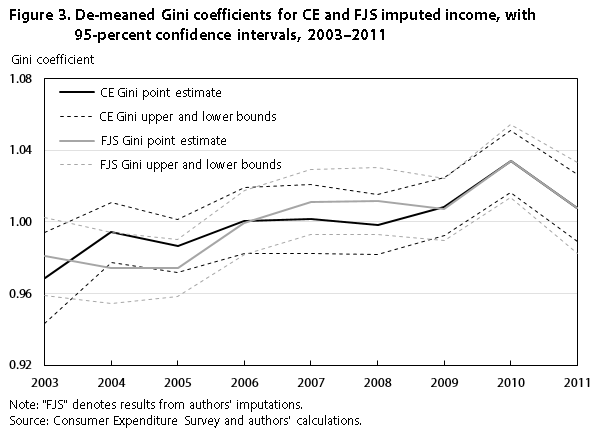
Figure 2 presents the Gini coefficient, which is a measure of income inequality. A Gini of 1.0 means complete inequality, whereas a Gini of 0.0 means complete equality. We present the Gini for the mean of the five implicates and the Gini for one of the implicates. As expected, the mean of the five implicates shows less inequality, because of a mean reversion resulting from averaging across the five implicates. Our Gini is below the CE Gini in some years but above it or right on in other years. Given the pattern in figure 1, where our 90th percentile value was lower than the CE’s 90th percentile value, we were concerned that our Gini would be consistently lower; however, this is not the case.
Figure 3 shows the de-meaned Gini coefficients,28 along with a 95-percent confidence interval. Although the levels of inequality for our imputed income and the CE imputed income are not identical, the difference is not statistically significant.
Figure 4 displays the full densities for our income variable and the CE income variable for 2009. The two variables largely overlap, except at the right tail of the distribution, matching the finding from figure 1. Another way to compare the distributions is with the scatterplot shown in figure 5. If our imputation matched the CE imputation exactly, all observations would lie along the 45-degree line displayed in the figure. Although the scatterplot is relatively tight along the 45-degree line, there are some outliers throughout the distributions. The correlation between the two income variables is .84.


Finally, we compare our imputed wage and salary income to that of the CE, presenting densities and a scatterplot analogous to those presented earlier. (See figures 6 and 7.) We focus on wage and salary income because it is the biggest source of income for most households. For this comparison, the unit of observation is the individual, not the household. Interestingly, our wage and salary distribution has a longer right tail than does the CE distribution, because we do not reimpose the top codes after imputation. The correlation between the two variables is .87.


The test in this first comparison shows only that our imputation matches the CE’s imputation. It does not indicate whether our imputation is accurate in itself. The next two comparisons help us determine the quality of our imputation.
Comparison 2—Imputing for valid reporters. In this comparison, we test how well our methodology imputes income for those in the CE who actually reported a valid value for an income source. For example, we take those who reported a valid nonzero value for wage and salary income in the first quarter of 2011 and treat them as if their income needed to be imputed. We use the previous 20 quarters of wage and salary reports and repeat the procedure for every income source and for every quarter.
With these new imputed values, we can compare the actual income reported in the CE to the imputed value. Because we are interested in total income and less so in the individual sources of income, we focus mainly on comparing total before-tax income. Therefore, our comparison includes those who reported a valid value for each source of income and had no imputation. We refer to this type of survey respondents as “full income reporters.” We might prefer to use the term “complete income reporters;” however, that term has its own confusing terminology in the CE lexicon. Our indicator of full income reporters is as strict as it can be—the household must have a valid report for each source of income. A zero can be a valid value.29
Figure 8 compares actual income of full income reporters with our imputation of all sources of income for these households at various points on the distribution. We do best at the mean and the 90th percentile, where our imputation is within 5 percent of the true value in all but 1 year for the mean and all but 3 years for the 90th percentile. In most years, our imputation is considerably higher at the 10th percentile, suggesting that we have difficulty imputing smaller values for those who received the income source. This pattern is different from that displayed in figure 1, where our imputation was right on at the 10th percentile but lower at the 90th percentile.
Figure 9 reports how well we match the trends in income inequality. The year 1993 is the only year for which the de-meaned trends show a statistically significant difference at the 5-percent level. The figure suggests that our imputation methodology does a decent job of capturing the de-meaned trends in inequality over the 1984–2011 period.
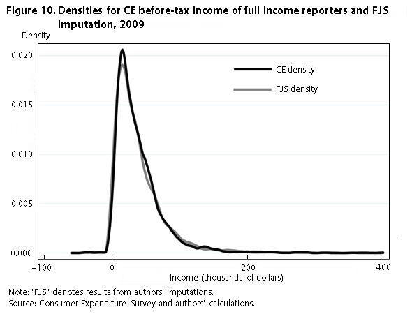
Figure 10 shows a pattern similar to that observed in figure 8. Our imputation is a little higher on the bottom end of the distribution but similar to CE income across the rest of the distribution. Compared with figure 5, the scatterplot for the two series in figure 11 shows more spread away from the 45-degree line, but the correlation coefficient between the two variables is still high, at .62.

Finally, figures 12 and 13 show the densities and the scatterplot, respectively, for wage and salary income in 2009 for full income reporters and our imputation. As before, the top-coding affects the full income reporters without constraining our imputed values for these individuals. This result explains both why our distributions have a longer right tail and the censoring seen on the x-axis in figure 13. The correlation between the two wage variables is relatively strong, with a correlation coefficient of .62.


Comparison 3—Comparison to the Current Population Survey. As a final test of the quality of our imputation, we compare our results to income from the CPS Annual Social and Economic Supplement (ASEC).30 When it comes to the collection of income data, the ASEC has two main advantages over the CE: (1) its focus is on income, whereas that of the CE is on expenditures; and (2) it has a larger sample size, allowing for more precise estimation.
Research that looks at income and consumption inequality usually uses the CPS for income.31 The CPS imputes income with the use of a “hot deck” methodology (i.e., duplication of other households’ responses). In the results presented here, we use imputed income from the CPS. For the CE, we revert to valid income values when these are reported by the household and to imputed values for invalid blanks. Although the CPS is not perfect, it does provide a point of comparison that is outside the CE.
Figure 14 compares our income measure to that of the CPS at various points on the distribution. For each of our four points, our imputed income is equal to or lower than income in the CPS. On average, our estimates are about 8 percent lower than the corresponding values in the CPS.
Figure 15 shows the de-meaned Gini coefficients from 1984 to 2011 for our imputation of CE income and the CPS income, along with the corresponding 95-percent confidence intervals. Except in 1994 and 2010, the two series exhibit no statistically significant difference, and their confidence intervals overlap. Choosing the end points as a frame of reference, we observe that, between 1984 and 2011, CPS income inequality increased by 8.1 percent while CE income inequality increased by 6.8 percent. However, it is not the case that the CE always shows a smaller increase in inequality, and choosing a different pair of years may produce a different result. For example, from 1984 to 2010, income inequality increased by 5.9 percent in the CPS and by 10.1 percent in the CE.
Figure 16 tells the same story as figure 14 does, showing that our imputed CE income is similar to the CPS income, except that our imputation is shifted to the left. Figure 17 shows the distributions of wage and salary income for the CPS and our imputed CE income. Although the CPS distribution has a longer right tail, the two densities generally overlap.


With this research, we provide a supplement to the public-use data of the CE Interview Survey by imputing income for those consumer units who failed to report a valid value for all of their income sources. We mimic the imputation methodology used by BLS as close as possible (with public-use data), and our series goes back to 1984 and continues through the latest year for which data are available. Eventually, we will make our data publicly available for researchers, and we hope to enlist BLS support to run similar imputations on the restricted-access CE data.
ACKNOWLEDGMENT: We would like to thank Laura Paszkiewicz and Geoffrey Paulin, both of the U.S. Bureau of Labor Statistics, for their help with income imputation.
Jonathan D. Fisher, David Johnson, and Timothy M. Smeeding, "Imputing income in the Consumer Expenditure Interview Survey," Monthly Labor Review, U.S. Bureau of Labor Statistics, November 2014, https://doi.org/10.21916/mlr.2014.37
1 See Orazio Attanasio, Erik Hurst, and Luigi Pistaferri, “The evolution of income, consumption, and leisure inequality in the US, 1980–2010,” working paper 17982 (National Bureau of Economic Research, 2012).
2 Income imputation refers to the process of estimating income values when they are not reported in the CE.
3 We have no plans to impute income in the CE Diary Survey.
4 See Jonathan Fisher, “Income imputation and the analysis of consumer expenditure data,” Monthly Labor Review, November 2006, pp. 11–19, https://www.bls.gov/opub/mlr/2006/11/art2full.pdf.
5 The term “complete income reporters” refers to survey respondents who provide sufficient income data for use in official publications.
6 Fisher, “Income imputation.”
7 See Jonathan Fisher, David Johnson, and Timothy Smeeding, “Inequality of income and consumption in the U.S.: measuring the trends in inequality from 1984 to 2011 for the same individuals,” Review of Income and Wealth (forthcoming, 2015). See also Jonathan Fisher, David Johnson, and Timothy Smeeding, “Exploring the divergence of consumption and income inequality during the Great Recession,” working paper presented at the 2014 American Economic Association Annual Meeting.
8 We use public-use CE files in this work. Although we report results through 2011, we are working on additional years of the CE Interview Survey, capturing data as they become available.
9 An “invalid nonresponse” is a nonresponse that is inconsistent with other data reported by the consumer unit. In the CE documentation, we impute income if the income source has a “B” or a “C” flag.
10 Before the third quarter of 1993, alimony and child support income were one variable. When feasible, the two income sources are treated separately, in accordance with the methodology described here.
11 Since the second quarter of 2001, the food stamp variable has included food stamps and electronic benefits. The variable also changed names at that time.
12 Lump-sum income includes lump-sum payments from estates, trusts, royalties, alimony, prizes, games of chance, and payments from people outside the consumer unit.
13 Before the second quarter of 2001, the food stamp variable did not allow for valid blanks, a flag code of “A”. Instead, consumer units were given a zero for the food stamp variable, and the flag indicated a valid value, a flag code of “D”. We treat these consumer units as “valid zeroes.”
14 The AVB process is not performed for wage and salary income, farm income or loss, and nonfarm business income or loss. If a respondent reports being employed but fails to report wage and salary income, he or she has an invalid blank and that source is imputed. If a respondent is not employed, he or she has a valid blank. Thus, a respondent with a valid blank for wage and salary income could not have received wage and salary income, because that individual was not working; hence, we refrain from changing the valid blank to an invalid blank. Similar logic applies to farm and nonfarm business income.
15 See Donald B. Rubin, Multiple imputation for nonresponse in surveys (New York: John Wiley and Sons, Inc., 1987).
16 It is understood that the CE program uses SAS for its imputation.
17 It is not known whether the CE program uses Ordinary Least Squares or another method to generate the coefficients.
18 For the family-level variables, the individual-specific demographic characteristics (e.g., age, race) are for the reference person.
19 The variable ERANKMTH is transformed with the use of the same methodology as that used to transform the dependent variables. Since the variable does not appear in the public-use files before the second quarter of 1994, the CE program office provided us with its values from 1987 to the first quarter of 1994. It also provided us with the variable's values from 2004 to 2006, because the values on file in this period are affected by imputation. For the 1984–1986 period, ERANKMTH was calculated from the MTAB file.
20 The variable for member-level race separated Asians from Pacific Islanders in the first quarter of 2003. To remain consistent, we grouped these two categories in all years. Also in the first quarter of 2003, the variable for race of the reference person included an additional category for “multiple races.” This coding was retained because it was not feasible to perform a recoding that would make the race variables agree.
21 Five categories were created for education: less than high school, high school, some college, college, and graduate degree.
22 Four categories were created for number of earners: 0, 1, 2, and 3+.
23 Additional occupational categories were included, starting in 1994. The categories were collapsed to match earlier data.
24 Although the CE program imputes income by family type (e.g., husband and wife with the youngest child under age 6, single men, single women), we do not. Instead, we include family type as an independent variable.
25 An additional category was added to the tenure variable in order to capture those in public housing or subsidized housing. The CE program has kept public housing and subsidized housing as separate categories in its imputations.
26 We use the state of residence if a value for it is provided and a dummy variable if the state is missing from the data.
27 In this comparison, we use the mean of the five implicates as our income variable. Results are similar when we use any of the individual implicates.
28 To obtain our de-meaned estimates, we divided the Gini coefficient in a given year by the mean of the Gini coefficients over the entire study period. Presenting de-meaned values allows us to focus on changes from the mean and permits a clearer illustration of observed trends.
29 AVBs are excluded from this exercise because they have no income to be imputed.
30 The CE program conducts its own comparison to the CPS. See “Measuring the impact of income imputation in the Consumer Expenditure Survey: a multi-year comparison of income data with estimates from the Current Population Survey,” report 1021 (U.S. Bureau of Labor Statistics, Consumer Expenditure Survey, 2006–2007), pp. 10–19, https://www.bls.gov/cex/twoyear/200607/csxcps.pdf.
31 See Bruce Meyer and James Sullivan, “Consumption and income inequality and the Great Recession,” American Economic Review 103, no. 3, 2013, pp. 178–183. See also Jonathan Heathcote, Fabrizio Perri, and Giovanni Violante, “Unequal we stand: an empirical analysis of economic inequality in the US, 1967–2006,” Review of Economic Dynamics 13, no. 1, 2010, pp. 15–51.