An official website of the United States government
An official website of the United States government
The .gov means it's official.
Federal government websites often end in .gov or .mil. Before sharing sensitive information,
make sure you're on a federal government site.
The site is secure.
The
https:// ensures that you are connecting to the official website and that any
information you provide is encrypted and transmitted securely.
“Western parents try to respect their children’s individuality, encouraging them to pursue their true passions, supporting their choices, and providing positive reinforcement and a nurturing environment. By contrast, the Chinese believe that the best way to protect their children is by preparing them for the future, letting them see what they’re capable of, and arming them with skills, work habits, and inner confidence that no one can ever take away.”
―Amy Chua, Battle Hymn of the Tiger Mother1
As an example shown by the excerpt from Chua’s book, recent popular literature discusses the varying perspectives on education by ethnicity and race and the ways in which families exert influence over educational choices.2 Higher education, after all, contributes to an individual’s capacity to earn a livelihood and improve his or her financial and social well-being, regardless of race or ethnicity.
In his book Human Capital, Nobel laureate economist Gary Becker3 articulated the premise that human capital arises out of any activity that increases individual productivity.4 Education is one such activity that increases the productivity of the individual, requiring the direct cost of the education (tuition, books, and housing) and the foregone earnings during education. In much the same way that a unit of physical capital such as production machinery generates a stream of production benefits (lightbulbs, automobiles, or basketballs) with market value, human capital that increases as a result of an investment in education will generate an augmented stream of earnings and social benefits that will accrue as long as the educational investment has market and social values.
Human capital is primarily produced in the family and in schools. According to Becker, parents’ altruistic investment in the child’s education depends on their willingness to forgo their own consumption for the sake of the child and on the likelihood that the investment will yield economic and intrinsic personal and social benefits for the child.
In addition, because education improves human capital, society accrues the benefits of a more productive workforce that contributes through specialization and innovation. Moreover, families accrue the direct and indirect benefits of family members who are more productive and better able to provide greater economic support to the family. Families that invest in the human capital of their children receive the social benefits of higher education, to include increased social opportunities and the positive social impression made by the individual and the family. The family is integral to the investment decision as well as the subsequent benefits to the child, the family, and society. In the words of Becker,5
“No discussion of human capital can omit the influence of families on the knowledge, skills, health, values, and habits of their children. Parents affect educational attainment, marital stability, propensities to smoke and to get to work on time, and many other dimensions of their children’s lives.”
At an individual and family level, various factors influence the level of education investment. These factors include the family socioeconomic status (such as the amount of disposable family income and the education level of the parents), the ability of the child to complete his or her education, and the perceived economic and social benefits. The weight given to investing in education is therefore related to not only the stream of economic benefits but also the underlying characteristics of the family that chooses to invest.
Drawing on evidence from the Bureau of Labor Statistics’ Consumer Expenditure Survey (CE) microdata, a household survey that provides information on the buying habits of American consumers, this study extends previous research on human capital and investment in education by examining differences in educational expenditure patterns between race and ethnicity. We disaggregate the investment decision into two separate stages and explore any differences at each stage. First is the decision to attend college. Second is the level of expenditures for education. An individual who decides to attend college may incur different costs, depending on the choice of an educational institution and family background. Studying the amount an individual spends, given his or her decision to attend college, may provide further insights into differences in the educational investment decision.
In this article, parent’s education level refers to the education level of the reference parent. With the release of 2012 CE data, education of reference person was replaced by highest education level of any member in the consumer unit. This newly defined education classification, although not used in the analysis herein, does not change any statistical significance of the results presented in this article.
Consequently, this article evaluates whether race and ethnicity contribute to differences in investments in higher education. An investment decision includes both the decision to attend college and the amount of money invested given that decision. Many studies stop at examining differences in the likelihood to attend college by race and ethnicity, yet many differences in investment may be uncovered in the level of expenditures decided on for higher education. In this article, we first review the discussion of returns to schooling and the decision to attend college. Next, we describe the dataset we use for analyses. Finally, we discuss in depth the pieces that make up the differences in an investment decision by examining the decision to attend college by race and ethnicity and then focusing on levels of expenditures differences for higher education.
Returns to schooling. The essence of human capital theory is that investments in human capital—schooling and training—raise a person’s income by increasing the individual’s productivity and in satisfying society’s demand for more highly remunerated skills. In the case of schooling, individuals forgo money they would have earned during their working years and instead incur direct educational costs to invest in their own human capital. The individual’s rate of return is based on the investment value of the gain in lifetime earnings.6
Other research focuses on the wide variety of forms returns to education can take, such as financial returns in the form of pay, nonmonetary opportunities such as more job and schooling options, and nonmarket returns; for example, the ability of the educated to use skills to perform services for themselves such as tax preparation that would otherwise be purchased.7 Although all of these benefits and those to society are important, the focus of human capital returns to schooling revolves around the lifetime earnings returns that come from additional education. A rich collection of studies provides estimates of returns to education dating from the late 1950s.8 These studies conclude that private rates of return vary by region, income grouping, and gender. In addition, rates of return are highest in primary education and diminish with additional years of education. In the United States, the overall (primary through higher education) private rate of return to investment in education is “on the order of 10 percent.”9
Other studies have considered race, ethnic, and gender differences in returns to schooling, in particular, higher education.10 The findings from many of these studies indicate that positive returns to education are common across races, ethnicities, and the two genders. Moreover, when differences in ability are considered, “little evidence of differences in the return to school across racial and ethnic groups” exists.11 Again, these studies, which employ different datasets at different times, estimate annual gains from education ranging from 6 percent to 15 percent.
Taken together, a human capital framework and the ensuing research lead to the following conclusions about the value of schooling:
· Additional years of schooling positively correlate with increased earnings. This relationship holds for primary, secondary, and higher education.
· The decision to invest in education is one that yields a wide range of benefits, including a positive rate of return for the individual and society.
· The private annual rate of return varies but generally ranges from 8 percent to 10 percent.
Decision to attend college. The likelihood of the decision to attend college hinges on the costs of and the perceived returns (whether financial or personal) to schooling, as just discussed. This decision is shown to influence conditions of the family significantly, such as income, wealth, and education level. Differences in college attendance by race and ethnicity have been well studied, but results vary.
Studies have shown that college attendance varies significantly by race and ethnicity. Without controlling for family background,12 studies have consistently found that Hispanic and African American families have lower levels of education and college attendance, while Asians tend to have higher levels of education and college attendance.13 The focus of many other studies has been on estimating the effect of family background factors in explaining differences in college attendance. These studies indicate a wide range of results in explaining college attendance gaps due to socioeconomic differences and academic achievement. Some studies show that socioeconomic differences explain all or at least a portion of the gap in college attendance. Other studies have also expanded the analysis and discussed differences in attendance between 2-year and 4-year colleges.
At one end of the spectrum, several studies indicated that—given similar academic achievement levels of the student and similar family backgrounds—young African Americans were more likely to attend college. Thomas Kane showed that at each Scholastic Assessment Test (SAT, formerly Scholastic Aptitude Test) level, African American student enrollment rates were higher than their White counterparts.14 Pamela Bennett and Yu Xie showed that African American students, compared with their White counterparts, are more likely to attend college, especially at low levels of family socioeconomic status.15 Audrey Light and Wayne Strayer showed that minorities are more likely than their White counterparts to attend colleges of all quality levels.16 Laura Walter Perna found that African Americans are about 11 percent more likely than Whites to enroll in a 4-year college or university in the fall after graduating from high school.17
Many studies indicate that college attendance differences are insignificant after accounting for family background factors. Kane and Spizman showed that lower average educational attainment of African Americans is the result of differences in parental income, education, and geographical location.18 Charles, Roscigno, and Torres showed that background inequalities explain the entire African American–White gap in the likelihood of college attendance.19 Sandra Black and Amir Sufi found that since the 1990s, at every point of the socioeconomic status, African Americans were no more likely to attend college than Whites.20 Two other studies have found that Hispanic high school graduates are as likely as Whites to attend college.21
Even at lower levels of significance, studies generally show that socioeconomic factors account for at least some of the difference in college attendance among races. Min Zhan and Michael Sherraden showed that when household assets are considered, a substantial portion of the African American–White gap in college attendance disappears.22
Regarding attendance at 2-year and 4-year institutions, Kao and Thompson found that although African American and Hispanic students are more likely to attend college than ever before, they are more likely than Whites or Asians to attend a 2-year college than a 4-year institution.23 Cameron and Heckman found that Hispanics show the highest 2-year entry rate compared with African Americans and Whites, which is partially attributable to the regional concentration of Hispanics in states, such as California and Texas, with extensive low-tuition community college networks.24
The analyses in this article are based on microdata from the Interview Survey of the CE of the U.S. Bureau of Labor Statistics (BLS). Data from the years 2008, 2009, and 2010 contain 90,872 observations taken from consumers who were interviewed between January 2008 and March 2011.25 Selected subsets of the complete dataset are used for various parts of our analyses. (See appendix A for number of observations for each subset.) CE interviews the sample family units on the basis of a rotating panel, surveying about 7,000 consumer units26 each quarter. Each consumer unit is interviewed once per quarter for up to five consecutive quarters. The Interview Survey is designed to capture expenditure data that respondents can reasonably recall for a period of 3 months or longer. In general, data captured include relatively large expenditures.27
This article examines the variation across consumer units, henceforth, “households,” at each interview, to explain differences in educational investment among racial groups and thus the article treats each household as a unique observation.28 All summary statistics, parameter estimates, and variances in this article are generated using weights created through balanced repeated replication, a procedure necessary to compute unbiased variance estimates through the CE’s use of a stratified random sample of geographic areas around the United States.29 The data represent the U.S. population in all analyses performed in this article. Results are derived with a SAS macro that the BLS developed.
To disaggregate educational expenditures, we provide a structure that outlines the decision to incur expenditures and describes how the CE data are organized in accordance with this structure. (See figure 1.) First, a qualified 16–24-year-old—one who graduated from high school but does not have a bachelor’s degree, henceforth, a “young adult,”—decides whether to go to college. Furthermore, if he or she decides to attend college, the educational expenditure may be made by the parent(s), young adult, both, or neither. For completeness, we discuss three types of households relevant to educational expenditures:
· Type 1—parent household without young adults residing in the household
· Type 2—young adult household
· Type 3—parent household with young adult(s) residing in the household

Households are identified as type 1 (78,686 observations) if no young adult member is acknowledged, during the interview, to reside in that household. Type 1 households include families (1) that do not have any young adult members (regardless of residence) and (2) those who have one (or more) young adult member(s) but who may be away (for college or living separately), although we cannot distinguish between these two subtypes in the data. Households identified as type 2 (4,099 observations) comprise young adult members who are the head of their household. This type includes those who are living apart30 from parents such as a college student. Type 3 (8,087 observations) households are identified as those with at least one young adult member who is not the head of a separate household and has at least one other older member (e.g., parent).
For type 1 households, we do not observe whether a young adult is away at college; we only know that, when we observe a positive expenditure for an unobserved individual who is away from home, an individual (likely to be a young adult) is away at college.31 For type 2 households, we observe the young adult’s college attendance decision32 and his or her own out-of-pocket expenditure for higher education. We do not, however, observe the young adult’s family background. For type 3 households, we observe both the young adult’s college attendance decision and the household expenditure for higher education.
Race and ethnicity. An individual’s race is identified as White, African American, Asian, or “other.” “Other” includes Native American, Pacific Islander, and multiracial. Ethnicity is classified as Hispanic and non-Hispanic. For the purpose of this article and because of limitations of sample size, Hispanic origin will be considered as a subset of only the White racial group. African American Hispanics and Asian Hispanics are grouped into “other.” Thus, the racial and ethnic groups used for this article are White (White non-Hispanics), Hispanics (White Hispanics), African Americans (African American non-Hispanics), Asians (Asian non-Hispanics), and other.33
Data control variables. To control for variations in the data that may inadvertently bias model results, we include indicators for year of interview, month of interview, month of expenditure, part-time student, and female.
Socioeconomic variables. For type 1 and type 3 households, factors associated with family background are observed, including education of the parent(s) and total outlays34 of the household, which is used as a proxy for permanent income.35 (See appendix B for more details.)
Other variables and model selection. Additional variables such as occupation and assets were available to be used in various parts of the analyses; however, the selection of covariates to use in each model was based on a combination of intuition and empiricism. Variables that had an economic relation and linearly related to the dependent variable were added to each model. Selection criteria36 were then applied and resulted in the final models that follows.
Prior to deciding on an amount to spend for higher education, individuals and families must first decide whether a member of the family is to attend college. As just discussed, the decision to attend is influenced by many factors, such as family income, race, their parents’ education, and wealth.
In our dataset, more than half of qualified young adults37 were in college, of which 83 percent were enrolled full time. Our data show that Hispanics (45 percent) and African Americans (43 percent) generally have lower college attendance rates than Whites (55 percent) or Asians (73 percent). As with previous studies, family background, such as their parents’ education and income, was significantly associated with the likelihood of attending college. As parent’s education level and income increase, the likelihood of a young adult attending college significantly increases. The extent to which socioeconomic differences explain differences in college attendance among racial and ethnic groups varies among models, but socioeconomic differences were generally found to account for some of the observed differences.38 (See appendix C, table C-1.) Part-time college attendance rates for Whites, African Americans, and Asians were between 7 percent and 8 percent, while Hispanics had a 14 percent part-time attendance rate. (See figures 2 and 3.)
At the aggregate level, as with published CE tables,39 Hispanic and African American households have a lower average household expenditure than White households do, whereas Asian households have a higher average household expenditure. (See table 1.) However, these overall averages are misleading, because they do not distinguish those students who are attending college from those who are not.
| Race or ethnicity | Mean | Standard error |
|---|---|---|
| White | 409.2 | 27.4 |
| Hispanic | 177.3 | 49.2 |
| African American | 125.3 | 18.5 |
| Asian | 644.3 | 112.1 |
Note: “Other” group is omitted. Source: U.S. Bureau of Labor Statistics. | ||
Once an individual has decided to attend college, he or she must decide on the amount to invest in higher education. In this section, we first discuss the characteristics of households with college-attending students. We then model the level of out-of-pocket tuition expenditures40 for those with a positive expenditure. Finally, we examine factors that are associated with a zero or unobserved out-of-pocket tuition expenditures.41
Profile of households with college-attending students. Among households with college-attending students, family characteristics vary significantly among racial and ethnic groups. Table 2 shows the characteristics of type 3 households—those with one or more parents and one or more students—by race and ethnicity in the dataset used for the analyses.
Education. Compared with Hispanic and African American parents, White and Asian parents of college-attending students have higher levels of education. Whereas 33 percent of White parents and 30 percent of Asian parents obtained a bachelor’s degree or higher, 18 percent of African American parents and 10 percent of Hispanic parents obtained the same degree. At the lower end of the education scale, 5 percent of White parents and 8 percent of Asian parents did not receive a high school diploma. In contrast, 12 percent of African American and 32 percent of Hispanic parents did not receive a high school diploma.
| Education of parents | White | Hispanic | African American | Asian |
|---|---|---|---|---|
| Less than high school (percent) | 5 | 32 | 12 | 8 |
| High school (percent) | 27 | 24 | 27 | 32 |
| Some college, associate’s degree (percent) | 36 | 34 | 42 | 30 |
| Bachelor’s degree (percent) | 23 | 7 | 13 | 17 |
| Graduate degree (percent) | 10 | 3 | 5 | 13 |
| Annual income (annualized total outlays) (dollars)(1) | 67,269 | 48,327 | 48,868 | 58,667 |
| Have any tuition expenditures (percent) | 28 | 18 | 14 | 28 |
| Average quarterly tuition (dollars) | 2,806 | 1,356 | 1,606 | 3,397 |
| Female student (percent) | 58 | 62 | 58 | 47 |
Notes: (1) Consumer unit type 3 households only (parents with young adults). Note: The term “total outlays” is a proxy for permanent income; we obtained annualized outlays by multiplying quarterly outlays by 4. Source: U.S. Bureau of Labor Statistics. | ||||
Income. Asian parents of college-attending students reported 13 percent less permanent income42 ($58,700) than White parents ($67,300). Relative to the income of White parents, Hispanic and African American parents had 28 percent and 27 percent less annual income, or $48,300 and $48,900, respectively.
Positive tuition expenditure. Asian households were as likely as White households to have a positive expenditure for education. However, Hispanics households were more than one-third less likely than White households to have a positive expenditure, while African Americans were only about half as likely.
Average tuition expenditure. Of the households with positive tuition expenditures, Asians reported 21 percent higher expenditures than Whites. Hispanics and African Americans reported 52 percent and 43 percent, respectively, lower expenditures than Whites reported.
While Hispanics and African Americans households with a student in college had, on average, a lower probability of having a positive expenditure and a lower amount of expenditure, they also had lower education and lower total outlays. To ascertain whether certain racial or ethnic groups tended to spend less (or more) on education because of their average socioeconomic differences, we performed a regression analysis.
Observed out-of-pocket tuition expenditures. We constructed a model for out-of-pocket positive tuition expenditures and used the method of ordinary least squares to estimate not only the relationship between race and ethnicity, but also socioeconomic characteristics, and the level of positive tuition expenditures. (See box that follows.)
Because expenditures are truncated at zero, are clustered around lower values, and have a long tail (are right-skewed), a transformation of the dependent variable is applied to approximate normality. For each model, an optimal Box-Cox transformation is applied to distribute tuition expenditures more normally and to stabilize variance.1
We start with an ordinary least squares model of (transformed) positive expenditures regressed on race and ethnicity, with data controls in which
 , (1)
, (1)
where Yλ is a vector of (transformed) observed tuition expenditure for higher education; X is a matrix of indicators for race and ethnicity; β is a vector of corresponding parameter estimates; Z is a matrix of data controls, including indicators for interview year, interview month, tuition expenditure month, female, and part-time student; γ is a vector of corresponding parameter estimates; and ε is a vector of errors.
We then add socioeconomic factors to equation (1), yielding
 , (2)
, (2)
where W is a vector of family background characteristics, including parent’s education level and annual permanent income,2 and η is a vector of corresponding parameter estimates.
Notes:
1 The optimal λ for consumer unit types 1, 2, and 3 are 0.12, 0.24, and 0.08, respectively.
2 The logarithm of income (annualized outlays) is used to overcome nonlinearity between permanent income and tuition expenditures.
The regression model results indicate significant differences in tuition expenditures by income, education, and race and ethnicity.
Income. Family income has a significant effect on educational expenditures. Ceteris paribus, for every $10,000 increase in annual permanent income, average annual tuition expenditures increase between $200 and $400 for type 1 households (parents without young adults) and between $120 and $360 for type 3 households (parents with young adults).43 (See appendix C, table C-2.)
Education. At household education levels of bachelor’s degree and below, differences in tuition expenditures are insignificant. On average, households with parents having a graduate degree had college tuition expenditures 40 percent to 80 percent higher than households with parents not having a graduate degree.44
Race and ethnicity. Differences in the level of expenditure for tuition are most pronounced for student-only households (type 2). Hispanic students, on average, spent half the amount that an average White student spent on tuition. On the other hand, Asians spent nearly twice as much as their White counterpart. However, the extent to which family characteristics explain the differences in expenditures remains uncertain for type 2 (student-only) households because these characteristics are unobserved in the data. Also, because of the small sample size of African American type 2 households, expenditure differences between this group and Whites are not statistically significant.
For parent-only (type 1) households, no significant differences in expenditures were found between racial and ethnic groups. For student and parent joint (type 3) households, Hispanics had 38 percent lower tuition expenditures than Whites. However, when controlling for the socioeconomic differences between Hispanics and Whites, we found that Hispanics’ lower expenditures were not statistically significant.45 This finding indicates that permanent income and education level effects accounted for nearly all the observed differences in tuition expenditures between Hispanics and Whites. (See table 3 and appendix C, table C-3.)
| Variable | Type 1 (model 1) | Type 1 (model 2) | Type 2 (model 1) | Type 3 (model 1) | Type 3 (model 2) |
|---|---|---|---|---|---|
| Race or ethnicity | |||||
Hispanic | –0.088 | –0.091 | –0.902 | –0.066 | –0.037 |
| (0.089) | (0.069) | (0.354)(1) | (0.020)(2) | (0.022)(3) | |
African American | 0.002 | 0.055 | –0.640 | –0.036 | –0.020 |
| (0.076) | (0.064) | (0.528) | (0.024) | (0.025) | |
Asian | 0.001 | 0.007 | 0.952 | 0.043 | 0.056 |
| (0.057) | (0.062) | (0.407)(1) | (0.028) | (0.033) | |
| Data controls | Yes | Yes | Yes | Yes | Yes |
| Socioeconomic controls | No | Yes(4) | No(5) | No | Yes |
Notes: (1) Significant at the 5-percent α level. (2) Significant at the 1-percent α level. (3) Significant at the 10-percent α level. (4) In-college part time and female not available. See appendix C, table C-3. (5) Socioeconomic controls not available. Note: Standard errors are in parenthesis. Type 1 is parent household without (visible) young adults, type 2 is young adult household, and type 3 is parent household with young adult(s). Model 1 does not include socioeconomic controls; model 2 includes socioeconomic controls. Source: U.S. Bureau of Labor Statistics. | |||||
Unobserved and zero out-of-pocket expenditures. The previous section addressed positive tuition expenditure differences, yet another important aspect to address is the likelihood of having a positive (and unobserved) expenditure.46A household with a young adult attending college may not have an observed positive expenditure for tuition. Many factors may prevent an expenditure from being observed. Examples include scholarships or some other financial aid covering all tuition fees,47 someone outside of the household covering the expenditure (especially for type 2 households), or someone covering a tuition expenditure in a month outside of the interview coverage months. Although the reasons for zero out-of-pocket expenditures are unknown in the data, we examine factors that are associated with the likelihood of having a positive tuition expenditure for types 2 and 3, the households in which a young adult in college is present. This last piece of modeling zero out-of-pocket expenditures is necessary and important to complete the analysis of investment in higher education. The box that follows describes our model for zero out-of-pocket tuition expenditures.
The response variable, regardless of whether a tuition expenditure is positive or zero, is a binary response. We use a logit1 model with data controls for type 2 and type 3 households as
 , (3)
, (3)
where T indicates positive tuition expenditure; X is a matrix of indicators for race and ethnicity; β is a vector of corresponding parameter estimates; Z is a matrix of data controls, including indicators for interview year, interview month, female, and part-time student; and γ is a vector of corresponding parameter estimates. The response in a logistic regression is modeled as log-odds, that is, the log of the ratio of the probability of a positive expenditure versus a zero expenditure.
For type 3 households, we then included socioeconomic controls as
 , (4)
, (4)
where in this equation, X, β, Z, and γ are as in equation (1); W is a matrix of family background characteristics, including parent’s education level and logarithm of total quarterly outlays, which are used as a proxy for permanent income; and η is a vector of corresponding parameter estimates.
Note:
1 We also used probit and linear probability models. The results were similar.
As with the results for the levels of expenditures, results obtained from models of zero expenditure indicate that income, education, and race and ethnicity are important determinates of whether a household will have positive expenditures.
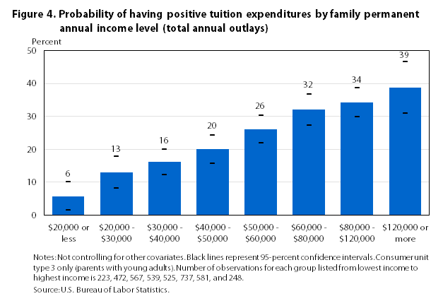
Income. Not surprisingly, permanent income is significantly associated with the likelihood of having any tuition expenditure. The probability of having out-of-pocket tuition expenditure increases with family income level. This relationship is expected because families with lower permanent income tend to receive more financial aid,48 increasing the likelihood of complete tuition coverage. Compared with families with an annual permanent income of $20,000 or less, families with $120,000 or more with a college-going child are about 6.5 times more likely to have tuition expenditure. (See figure 4.) Even after controlling for other covariates, such as race, other socioeconomic factors, and data controls, the income effect remains highly significant. (See appendix C, table C-2.)
Education. As expected, as parents’ education level increases, the probability of having positive tuition expenditure increases. (See figure 5.) Even when other factors such as permanent income are controlled, the probability still increases with education level.49 (See appendix C, table C-2, for results obtained from the model.)
Race and ethnicity. Even when differences in family background are controlled, our model yields results which indicate that, of those households with one or more members who attend college, African American households are significantly less likely to have an observed positive expenditure for tuition compared with White households. Asian households show a marginally significantly higher probability of having a positive expenditure.50 (See table 4 and appendix C, table C-2.)
| Variable | Type 2 (model 3): without socioeconomic controls | Type 3 (model3): without socioeconomic controls | Type 3 (model 4): with socioeconomic controls |
|---|---|---|---|
| Race or ethnicity | |||
Hispanic | 0.134 | –0.194 | –0.029 |
| (0.203) | (0.160) | (0.151) | |
African American | –1.154 | –0.560 | –0.476 |
| (0.309)(1) | (0.176)(2) | (0.163)(2) | |
Asian | 0.648 | 0.279 | 0.233 |
| (0.336)(3) | (0.141)(4) | (0.124)(3) | |
| Data controls | Yes | Yes | Yes |
| Socioeconomic controls | No(5) | No | Yes |
Notes: (1) Significant at the 0.1-percent α level. (2) Significant at the 1-percent α level. (3) Significant at the 10-percent α level. (4) Significant at the 5-percent α level. (5) Socioeconomic controls not available. Note: Standard errors are in parenthesis. Type 2 is young adult household, and type 3 is parent household with young adult(s). Source: U.S. Bureau of Labor Statistics. | |||
DIFFERENCES IN INVESTMENT IN HIGHER EDUCATION between racial and ethnic groups arise from differences in college attendance, the level of expenditures for higher education and, to a greater extent, the likelihood of having positive education expenditures. Some of the differences, as shown in table 5, can be attributed to differences in family socioeconomic status, such as parent’s education level and permanent income. In narrative terms, our results are as follows:

· Relative to White households, Hispanic households tend to have lower rates of college attendance and some evidence shows lower levels of tuition expenditures, as well. Our results indicate that the overall lower levels of household tuition expenditures for Hispanics are due primarily to generally lower levels of permanent income, parent’s education level, the decision to attend college and, to some extent, the levels of tuition expenditure of students. However, after accounting for differences in education and permanent income, Hispanic households do not differ significantly either in the likelihood of having any tuition expenditures or in the level of expenditures.
· African American young adults tend to have lower rates of college attendance and, among those who decide to attend college, a lower probability of having any tuition expenditure, even when family permanent income and education level are considered. However, of those who have any tuition expenses, the levels of expenditures are not significantly different from those of White families. The primary contributing factors to lower levels of household tuition expenditure by African Americans are socioeconomic differences, a lower likelihood to attend college, and the higher likelihood of having no expenditures even when one decides to attend college.
· Asian young adults have higher rates of college attendance than any other race or ethnicity. Asian parents do not have a significantly higher level of tuition expenditures. However, some evidence points to higher levels of expenditures from students in student-only households. These results suggest that Asian households’ overall higher expenditures for education are primarily due to the higher rates of college attendance in Asian families, and, to some extent, the higher levels of tuition expenditures by Asian student-only households.
With a variety of factors contributing to the overall decision of college investment, differences arise among racial and ethnic groups. Notwithstanding the complexity of socioeconomic factors, our findings suggest that differences in permanent income and education level of parents are important in the decision to attend college, in the level of expenditures, and in the likelihood of having a positive expenditure for education. Controlling for these important factors, we find that whereas the decision whether to invest may be different for Asians, African Americans, and Hispanics, the amount of investment, for the most part, is not significantly different from that of Whites.
Previous studies have shown that similar returns to schooling exist across different races and ethnicities, even if the likelihood to attend college is different. However, given the decision to invest and given evidence of positive expenditures, we found no significant differences in the level of investment. These results suggest that, although the perceived returns to schooling may be different for different races and ethnicities, the investment value of education for those who choose to invest is unambiguous, both in perception and in effect. Returning to the earlier discussion of higher education and human capital, we conclude that once a decision to invest in higher education is made and positive expenditures are registered by a family, little difference exists in the amount for education investments between the racial and ethnic groups studied. In other words, we find that all racial and ethnic groups believe in and invest in the human capital idea that investments in higher education are economically beneficial to their children.
The authors would like to thank BLS Senior Economist Geoffrey Paulin from the Office of Prices and Living Conditions for his invaluable comments, review, guidance, and patience through many revisions of this article; BLS Branch Chief and Supervisory Economist Steve Henderson, BLS Supervisory Economist Bill Passero, and BLS Economists Adam Reichenberger and Lucilla Tan, all also from the Office of Prices and Living Conditions; BLS Supervisory Economist Martin Kohli from the New York Regional Office for Economic Analysis and Information, BLS Deputy Associate Commissioner Michael Strople from the Office of Field Operations, BLS Supervisory Economist Amar Mann from the San Francisco Regional Office, BLS Associate Commissioner Jay Mousa from the Office of Field Operations, and Research Economist Harley Frazis from the Office of Employment and Unemployment Statistics, for their review and comments; and Regina Wu, formerly an intern at BLS, for her research assistance, comments, and review.
| Race or ethnicity | All observations by type | In college by type | Observed positive tuition expenditure by type | |||||
|---|---|---|---|---|---|---|---|---|
| 1 | 2 | 3 | 2 | 3 | 1 | 2 | 3 | |
White | 55,301 | 2,956 | 4,539 | 2,070 | 2,192 | 868 | 476 | 644 |
Hispanic | 8,951 | 404 | 1,707 | 165 | 783 | 41 | 28 | 130 |
African American | 9,126 | 454 | 1,130 | 205 | 485 | 47 | 13 | 66 |
Asian | 3,608 | 169 | 461 | 144 | 314 | 57 | 41 | 88 |
Other | 1,700 | 116 | 250 | 71 | 118 | 12 | 10 | 29 |
Total | 78,686 | 4,099 | 8,087 | 2,655 | 3,892 | 1,025 | 568 | 957 |
Note: Type 1 is parent household without young adults, type 2 is young adult household, and type 3 is parent household with young adult(s). Source: U.S. Bureau of Labor Statistics. | ||||||||
| Variable | Values and range | Notes |
|---|---|---|
Consumer unit type
| 1: No qualified 16–24-year-old in consumer unit | Consumer unit type |
| 2: Qualified 16–24-year-old without parent(s) in consumer unit | ||
| 3: Qualified 16–24-year-old with parent(s) in consumer unit | ||
In college
| 1: In college full time | For qualified 16–24-year-olds only |
| 2: In college part time | ||
| 3: Not in college | ||
Tuition expenditure for higher education | [$0, ∞) ϵ ℝ | Quarterly expenditure |
Tuition indicator
| 1: Tuition > 0 | — |
| 0: Tuition = 0 or blank | ||
Tuition expenditure month | [1, 13] ϵ ℕ | Month in which the expenditure was made; month 13 indicates same amount each month |
Race and ethnicity
| 1: White non-Hispanic | Race and ethnicity of head of household; other includes Native American, Pacific Islander, and multiracial |
| 2: White Hispanic | ||
| 3: African American non-Hispanic | ||
| 4: Asian non-Hispanic | ||
| 5: Other | ||
Female
| 0: Male | Gender of qualified 16–24-year-olds |
| 1: Female | ||
Year | [2008, 2011] ϵ ℕ | Year of interview |
Interview month | [1, 12] ϵ ℕ | Month in which the interview was conducted |
Education level
| 1: No high school graduate | For types 1 and 3 consumer unit head of households only |
| 2: High school graduate | ||
| 3: Some college, associate’s degree | ||
| 4: Bachelor’s degree | ||
| 5: Master’s, professional, or doctorate degree | ||
Total outlays less tuition expenditures for higher education | [$0, ∞) ϵ ℝ | Quarterly outlays; for types 1 and 3 consumer unit head of households only; proxy for permanent income |
| Source: U.S. Bureau of Labor Statistics. | ||
| Variable | Type 3: without socioeconomic covariates | Type 3: with socioeconomic covariates | ||
|---|---|---|---|---|
| Estimate | Standard error | Estimate | Standard error | |
Intercept | 0.047 | (0.065) | –3.027 | (0.840)(1) |
Hispanic | –.206 | (.131) | –.037 | (.138) |
African American | –.315 | (.113)(2) | –.249 | (.114)(3) |
Asian | .737 | (.149)(1) | .634 | (.157)(1) |
Other | –.089 | (.246) | –.077 | (.267) |
Interview year | ||||
2008 | –.228 | (.064)(1) | –.229 | (.066)(1) |
2009 | –.062 | (.052) | –.061 | (.055) |
2000 | .134 | (.044)(2) | .151 | (.046)(1) |
Interview month | ||||
January | –.015 | (.061) | –.027 | (.061) |
February | –.059 | (.057) | –.051 | (.061) |
March | –.056 | (.065) | –.061 | (.066) |
April | –.034 | (.066) | –.032 | (.072) |
May | .028 | (.082) | .040 | (.083) |
June | .059 | (.074) | .060 | (.074) |
July | –.122 | (.064)(4) | –.136 | (.067)(3) |
August | .019 | (.061) | .042 | (.065) |
September | .040 | (.078) | .005 | (.074) |
October | .013 | (.066) | .014 | (.074) |
November | .024 | (.068) | .042 | (.070) |
Education | ||||
Less than high school | — | — | –.538 | (.084)(1) |
High school | — | — | –.279 | (.078)(1) |
Some college, associate’s degree | — | — | .064 | (.066) |
Graduate degree | — | — | .472 | (.142)(1) |
Log income | — | — | .340 | (.091)(1) |
Notes: (1) Significant at the 0.1-percent α level. (2) Significant at the 1-percent α level. (3) Significant at the 5-percent α level. (4) Significant at the 10-percent α level. Note: Type 3 is parent household with young adult(s). Source: U.S. Bureau of Labor Statistics. | ||||
| Variable | Type 1 (model 1) | Type 1 (model 2) | Type 2 (model 1) | Type 3 (model 1) | Type 3 (model 2) | |||||
|---|---|---|---|---|---|---|---|---|---|---|
| Estimate | Standard error | Estimate | Standard error | Estimate | Standard error | Estimate | Standard error | Estimate | Standard error | |
Intercept | 2.239 | (0.105)(1) | 0.383 | (0.293) | 5.543 | (0.718)(1) | 1.777 | (0.051)(1) | 1.310 | (0.145)(1) |
Hispanic | –.088 | (.089) | –.091 | (.069) | –.902 | (.354)(2) | –.066 | (.020)(3) | –.037 | (.022)(4) |
African American | .002 | (.076) | .055 | (.064) | .640 | (.528) | –.036 | (.024) | –.020 | (.025) |
Asian | .001 | (.057) | .007 | (.062) | .952 | (.407)(2) | .043 | (.028) | .056 | (.033) |
Other | .045 | (.188) | .081 | (.142) | .717 | (.510) | –.095 | (.042)(2) | –.073 | (.041)(4) |
Interview year | ||||||||||
2009 | .035 | (.059) | .041 | (.059) | –.326 | (.349) | –.020 | (.028) | –.010 | (.023) |
2010 | .033 | (.061) | .015 | (.064) | –.114 | (.382) | –.016 | (.033) | –.003 | (.029) |
2011 | .026 | (.059) | .020 | (.056) | –.230 | (.505) | –.007 | (.027) | .006 | (.022) |
Interview month | ||||||||||
January | .054 | (.092) | .031 | (.086) | .368 | (.809) | –.020 | (.051) | –.015 | (.053) |
February | .155 | (.089)(4) | .119 | (.078) | –.784 | (.621) | –.001 | (.039) | .002 | (.039) |
March | .020 | (.082) | –.007 | (.075) | –.991 | (.659) | –.027 | (.039) | –.024 | (.038) |
April | .019 | (.099) | .026 | (.086) | –.751 | (.638) | –.015 | (.038) | –.005 | (.037) |
May | .041 | (.110) | .027 | (.104) | –.992 | (.651) | –.018 | (.049) | –.011 | (.050) |
June | –.107 | (.092) | –.096 | (.085) | –.091 | (.580) | –.060 | (.040) | –.047 | (.038) |
July | –.031 | (.095) | –.024 | (.090) | –.050 | (.608) | –.122 | (.055)(2) | –.125 | (.052)(2) |
August | –.009 | (.096) | –.017 | (.086) | .082 | (.749) | –.048 | (.050) | –.044 | (.049) |
September | .021 | (.069) | .025 | (.064) | –.186 | (.580) | –.051 | (.033) | –.047 | (.029) |
October | .005 | (.077) | .016 | (.066) | .082 | (.522) | –.044 | (.035) | –.041 | (.033) |
November | .020 | (.064) | .027 | (.058) | –.028 | (.547) | –.035 | (.030) | –.035 | (.027) |
Expenditure month | ||||||||||
January | .267 | (.050)(1) | .233 | (.049)(1) | 1.647 | (.375)(1) | .069 | (.025)(3) | .073 | (.023)(3) |
February | .055 | (.065) | .034 | (.058) | .090 | (.586) | .034 | (.023) | .035 | (.021) |
March | .205 | (.060)(3) | .200 | (.057)(3) | .490 | (.773) | .037 | (.030) | .030 | (.030) |
April | .224 | (.066)(3) | .189 | (.061)(3) | .171 | (.444) | .057 | (.035) | .051 | (.035) |
May | .113 | (.068) | .088 | (.062) | –.650 | (.573) | .041 | (.030) | .036 | (.029) |
June | .084 | (.061) | .046 | (.052) | –.245 | (.310) | .099 | (.032)(3) | .104 | (.030)(3) |
July | .279 | (.056)(1) | .257 | (.046)(1) | .369 | (.669) | .094 | (.042)(2) | .077 | (.040)(4) |
August | .294 | (.048)(1) | .231 | (.044)(1) | 1.129 | (.601)(4) | .097 | (.026)(1) | .095 | (.027)(1) |
September | .210 | (.051)(1) | .171 | (.043)(1) | .418 | (.402) | .073 | (.029)(2) | .074 | (.029)(2) |
October | .141 | (.053)(2) | .133 | (.043)(3) | .282 | (.484) | .016 | (.032) | .023 | (.031) |
November | –.017 | (.061) | –.025 | (.057) | .604 | (.588) | –.039 | (.041) | –.033 | (.040) |
December | .273 | (.047)(1) | .265 | (.043)(1) | .481 | (.419) | .072 | (.015)(1) | .065 | (.014)(1) |
In college part time | — | — | — | — | –.912 | (.282)(3) | –.080 | (.017)(1) | –.067 | (.019)(3) |
Female | — | — | — | — | .028 | (.156) | –.014 | (.013) | –.011 | (.013) |
Education | ||||||||||
Less than high school | — | — | –.014 | (.070) | — | — | — | — | –.007 | (.032) |
High school | — | — | –.024 | (.044) | — | — | — | — | –.003 | (.016) |
Some college, associate’s degree | — | — | .095 | (.028)(3) | — | — | — | — | .062 | (.018)(3) |
Graduate degree | — | — | .161 | (.046)(3) | — | — | — | — | .076 | (.022)(3) |
Log income | — | — | .183 | (.028)(1) | — | — | — | — | .043 | (.016)(3) |
Notes: (1) Significant at the 0.1-percent α level. (2) Significant at the 5-percent α level. (3) Significant at the 1-percent α level. (4) Significant at the 10-percent α level. Note: Type 1 is parent household without young adults, type 2 is young adult household, and type 3 is parent household with young adult(s). Model 1 does not include socioeconomic controls; model 2 includes socioeconomic controls. Source: U.S. Bureau of Labor Statistics. | ||||||||||
| Variable | Type 2 (model 3) | Type 3 (model 3) | Type 3 (model 4) | |||
|---|---|---|---|---|---|---|
| Estimate | Standard error | Estimate | Standard error | Estimate | Standard error | |
Intercept | –1.906 | (0.254)(1) | –1.257 | (0.101)(1) | –8.325 | (0.971)(1) |
Hispanic | .134 | (.203) | –.194 | (.160) | –.029 | (.151) |
African American | –1.154 | (.309)(1) | –.560 | (.176)(2) | –.476 | (.163)(2) |
Asian | .648 | (.336)(3) | .279 | (.141)(4) | .233 | (.124)(3) |
Other | –.050 | (.453) | .082 | (.183) | .044 | (.195) |
In college part time | –.042 | (.179) | –.474 | (.145)(2) | –.358 | (.153)(4) |
Female | .033 | (.162) | –.094 | (.090) | –.066 | (.096) |
Interview year | ||||||
2008 | .205 | (.131) | .072 | (.091) | .079 | (.092) |
2009 | .091 | (.095) | .158 | (.071)(4) | .181 | (.072)(4) |
2000 | –.023 | (.135) | –.117 | (.055)(4) | –.094 | (.057)(3) |
Interview month | ||||||
January | –.477 | (.317) | –.250 | (.156) | –.295(1) | (.156)(3) |
February | .709 | (.221)(2) | .361 | (.145)(4) | .461 | (.155)(2) |
March | .452 | (.151)(2) | .465 | (.120)(1) | .471 | (.126)(1) |
April | .337 | (.209) | .287 | (.142)(4) | .293 | (.149)(4) |
May | –1.011 | (.315)(2) | –.937 | (.147)(1) | –.912 | (.151)(1) |
June | –.372 | (.394) | –.481 | (.161)(2) | –.505 | (.170)(2) |
July | .268 | (.245) | –.183 | (.099)(3) | –.248 | (.104)(4) |
August | –.479 | (.534) | –.599 | (.170)(1) | –.584 | (.166)(1) |
September | .283 | (.146)(3) | .453 | (.129)(1) | .413 | (.134)(2) |
October | .550 | (.190)(2) | .568 | (.123)(1) | .528 | (.130)(1) |
November | .405 | (.154)(2) | .541 | (.138)(1) | .611 | (.138)(1) |
Education | ||||||
Less than high school | — | — | — | — | –.382 | (.176)(4) |
High School | — | — | — | — | –.236 | (.096)(4) |
Some college, associate’s degree | — | — | — | — | .031 | (.087) |
Graduate degree | — | — | — | — | .469 | (.178)(2) |
Log income | — | — | — | — | .745 | (.100)(1) |
Notes: (1) Significant at the 0.1-percent α level. (2) Significant at the 1-percent α level. (3) Significant at the 10-percent α level. (4) Significant at the 5-percent α level. Note: Type 2 is young adult household and type 3 is parent household with young adult(s). Model 3 does not include socioeconomic controls; model 4 includes socioeconomic controls. Source: U.S. Bureau of Labor Statistics. | ||||||
Tian Luo and Richard J. Holden, "Investment in higher education by race and ethnicity," Monthly Labor Review, U.S. Bureau of Labor Statistics, March 2014, https://doi.org/10.21916/mlr.2014.9
1 New York: Penguin Press, 2011.
2 See also Sandra Tsing Loh, “My Chinese American problem—and ours,” The Atlantic Monthly, April 2011, p. 83–91.
3Gary S. Becker, Human Capital: a theoretical and empirical analysis, with special reference to education, 3rd ed. (Chicago, IL, University of Chicago Press, 1994).
4 Jacob Mincer’s book Schooling, experience, and earnings (New York: Columbia University Press, 1974) is also credited with providing a theoretical and empirical basis for evaluating human capital and earnings.
5Gary S. Becker, “Human capital,” in David R. Henderson, The concise encyclopedia of economics, Library of Economics and Liberty (Indianapolis: Liberty Fund, 2008), http://www.econlib.org/library/Enc/HumanCapital.html.
6Societies invest in human capital in the form of educational facilities, programs, and subsidies. The social rate of return is based on the benefits to society of having a more highly educated workforce, less the cost of providing the educational services required to achieve those benefits. In evaluating the rate of return to schooling, human capital theory factors in the effects of cognitive ability and technological change on individual human capital and economic growth. Briefly, the reasoning is that the cognitive ability of the individual contributes to the returns to schooling because those with higher cognitive abilities select schooling over paid work, and therefore, the observed returns actually relate to the individual’s innate abilities rather than the level of schooling. The difficulty in distinguishing the contribution of ability from that of schooling has led some economists to conclude that “education and cognitive ability are so strongly associated that the wage effects of the two cannot be separated for all groups . . . . The real problem is that ability and schooling appear to be inseparable—all interaction and not main effects—even if ability is perfectly observed.” See James Heckman and Edward Vytlacil, “Identifying the role of cognitive ability in explaining the level of and change in the return to schooling,” Working Paper 7820 (Cambridge, MA: National Bureau of Economic Research, August 2000), p. 18. Other researchers have also evaluated the effects of “signaling” ability on rates of return to schooling. The idea is that, in the absence of another tangible measure of ability, achievements in higher education allow employers to sort prospective employees on the basis of the presumed “signal” that the individual has enhanced productivity. A National Bureau of Economic Research study concluded that although high school graduates returns to ability are negligible, college graduation “plays more than just a signaling role in the determination of wages. . . . Graduation from colleges allows individuals to directly reveal their ability to potential employers.” In other words, differences in ability do not lead to significant wage differences for high school graduates without experience but are more tangible among college graduates and are reflected in differences in wages. Moreover, among college graduates, no estimated differences exist in wages or returns to ability by race. For more information, see Peter Arcidiacono, Patrick Bayer, and Aurel Hizmo, “Beyond signaling and human capital: education and revelation of ability,” Working Paper 13951 (Cambridge, MA: National Bureau of Economic Research, April 2008).
7Burton A. Weisbrod, “Education and investment in human capital,” part 2, “Investment in human beings,” Journal of Political Economy, October 1962, pp. 106–123.
8 For a useful survey of studies in various countries over nearly 50 years, see George Psacharopoulos and Harry Anthony Patrinos, “Returns to investment in education: a further update,” Education Economics 12, no. 2 (September 2002), pp. 111–134.
9 Ibid., p. 116.
10 Fred Hines, Luther Tweeten, and Martin Redfern, “Social and private rates of return to investment in schooling, by race-sex groups and regions,” Journal of Human Resources, Summer 1970, pp. 318–340; Susan Averett and Sharon Dalessandro, “Racial and gender differences in the returns to 2-year and 4-year degrees,” Education Economics, March 2001, pp. 281–292; Lisa Barrow and Cecilia Elena Rouse, “Do returns to schooling differ by race and ethnicity?” Working Paper 2005-02 (Federal Reserve Bank of Chicago, February 2005), pp. 34; and Lisa Barrow and Cecilia Elena Rouse, “The economic value of education by race and ethnicity,” Economic Perspectives, 2Q/2006 (Federal Reserve Bank of Chicago, 2006), pp. 14–27.
11 Barrow and Rouse, “The economic value of education,” p. 23.
12 Family background, or socioeconomic factors, may be captured through a variety of proxies, such as income, wealth, education, etc.
13 See Current Population Survey (CPS): Statistical abstract of the United States: 2012, “Table 229. Educational attainment by race and Hispanic origin: 1970 to 2010” and “Table 230. Educational attainment by race, Hispanic origin, and sex: 1970 to 2010” (U.S. Census Bureau, 2012), https://www.census.gov/compendia/statab/2012/tables/12s0229.pdf; and Economic news release: college enrollment and work activity of high school graduates new release (U.S. Bureau of Labor Statistics, April 8, 2011), https://www.bls.gov/news.release/archives/hsgec_04082011.htm.
14 Thomas J. Kane, “Race, college attendance, and college completion” (U.S. Department of Education, 1994), http://eric.ed.gov/?id=ED374766.
15 Pamela R. Bennett and Yu Xie, “Revisiting racial differences in college attendance: the role of historically Black colleges and universities,” American Sociological Review, August 2003, pp. 567–580.
16 Audrey Light and Wayne Strayer, “From Bakke to Hopwood: does race affect college attendance and completion?” Review of Economics and Statistics 84, February 2002, pp. 34–44.
17 Laura Walter Perna, “Differences in the decision to attend college among African Americans, Hispanics, and Whites,” The Journal of Higher Education special issue: “The shape of diversity” (March 2000), pp. 117–141.
18 Thomas J. Kane and Lawrence. M. Spizman, “Race, financial aid awards, and college attendance,” American Journal of Economics and Sociology, January 1994, pp. 85–96.
19 Camille Z. Charles, Vincent J. Roscigno, and Kimberly C. Torres, “Racial inequality and college attendance: the mediating role of parental investments,” Social Science Research 36, March 2007, pp. 329–352.
20 Sandra E. Black and Amir Sufi, “Who goes to college—differential enrollment by race and family background,” Working Paper No. 9310 (National Bureau of Economic Research, November 2002).
21 Philip T. Ganderton and Richard Santos, “Hispanic college attendance and completion: evidence from the high school and beyond surveys,” Economics of Education Review 14, March 1995, pp. 35–46; and Perna, “Differences in the decision to attend college.”
22 Min Zhan and Michael Sherraden, “Assets and liabilities, race/ethnicity, and children’s college education,” Children and Youth Services Review, November 2011, pp. 2168–2175.
23Grace Kao and Jennifer S. Thompson, “Racial and ethnic stratification in educational achievement and attainment,” Annual Review of Sociology, August 2003, pp. 417–442.
24 Stephen V. Cameron and James J. Heckman, “The dynamics of educational attainment for Black, Hispanic, and White males,” Journal of Political Economy 109, June 2001, pp. 455–499.
25 Expenditures refer to October 2007 through December 2010.
26 A consumer unit comprises (1) all members of a particular household who are related by blood, marriage, adoption, or other legal arrangements; (2) a person living alone or sharing a household with others or living as a roomer in a private home or lodging house or in permanent living quarters in a hotel or motel but who is financially independent; or (3) two or more persons living together who use their income to make joint expenditure decisions. The three major expense categories that determine financial independence are housing, food, and other living expenses. To be considered financially independent, the respondent has to provide, entirely or in part, at least two of the three major expense categories.
27 For more information on expenditures, see “Appendix A: description of the Consumer Expenditure Survey,” Consumer Expenditure Anthology, 2011, Report 1030 (U.S. Bureau of Labor Statistics, July 2011), pp. 47–48, https://www.bls.gov/cex/anthology11/csxanthol11.pdf.
28 A unique observation is also known as a “unique NEWID.” NEWID is a global identifier in CE, which identifies each observational unit.
29 For more details on balanced repeated replication, see David Swanson’s “Standard errors in the 2011 Consumer Expenditure Survey” (U.S. Bureau of Labor Statistics, 2011), https://www.bls.gov/cex/ce_se_2011.pdf.
30 The word “apart” signifies that the young adult does not live in the same household as the parent(s).
31 Tuition expenditures of type 1 households for the individual not seen in the household are captured through a gift code, indicating whether the expenditure was for someone outside of the household and whether it was an expenditure for college. We do not know, however, the age of the individual for whom the expenditure was made.
32 Data are captured through the code designating “in college full or part-time or not in college code.”
33 “Other” includes Native American (Hispanic and non-Hispanic), Pacific Islander (Hispanic and non-Hispanic), multiracial (Hispanic and non-Hispanic), African American Hispanic, and Asian Hispanic. For African Americans and Asians, individuals of Hispanic origin consisted of less than 2 percent of each population.
34 Total outlays less tuition expenditures for higher education were used throughout this article. (See appendix B in this article for details.)
35 According to the “permanent-income hypothesis,” expenditures are made on the basis of levels of wealth rather than current income. Thus, total outlays indicate a consumer’s tastes and preferences better than current income does. See Milton Friedman, A Theory of the Consumption Function (Princeton, NJ: Princeton University Press, 1957), p. 6.
36 Based on Akaike information criterion (AIC), similar results were found with Bayesian information criterion (BIC), also known as the Schwarz criterion.
37 Young adults were from type 2 and type 3 households, only.
38 Results are based on logit models of college attendance on race, data controls, and family socioeconomic factors for type 3 households. Asians were consistently found to have a significantly higher likelihood of going to college, regardless of any socioeconomic differences. For Hispanics and African Americans, socioeconomic factors explained some but not all of the difference in their lower likelihood of attending college. (See appendix C, table C-1.)
39 For more information, see “Table 2100. Race of reference person: average annual expenditures and characteristics, Consumer Expenditure Survey, 2008” (U.S. Bureau of Labor Statistics), https://www.bls.gov/cex/2008/Standard/race.pdf; Table 2100. Race of reference person: average annual expenditures and characteristics, Consumer Expenditure Survey, 2009” (U.S. Bureau of Labor Statistics, October 2010), https://www.bls.gov/cex/2009/Standard/race.pdf; and “Table 2100. Race of reference person: average annual expenditures and characteristics, Consumer Expenditure Survey, 2010” (U.S. Bureau of Labor Statistics, September 2011), https://www.bls.gov/cex/2010/Standard/race.pdf.
40 Our analyses also considered other expenses for higher education, such as room and board, textbooks. However, we did not observe any significant differences by race and ethnicity. Thus, we focused our study of expenditures on tuition only. The results using total expenditures, including other expenses for college, were similar.
41 Because of the limitations of the data, we could not explicitly account for differences in the amount of financial aid received across race and ethnicity, which may affect the levels and likelihood of an out-of-pocket tuition expenditure. A study showed that, except for Asian students, White students receive the least amount of financial aid; see Susan Borowski, “Scholarships and the White male: disadvantaged or not?” Insight into Diversity, April to May 2012, pp. 14–17, http://unival.com/PDF/InsightIntoDiversityMagazine_April-May%20Issue.pdf.
42 Data are based on quarterly outlays multiplied by 4.
43 Estimates were evaluated at annual permanent income levels between $20,000 and $120,000 for the baseline group, i.e., White, male student, parent with a bachelor’s degree, with default data controls.
44 Data were estimated for White households with a male student and an average annual income of $70,000, with default data controls.
45 Expenditures were evaluated with default data controls, as usual.
46 Zero expenditures, or “inhibitions” to observing a positive expenditure, are essentially the first hurdle to overcome in a variation of a double-hurdle model. However, in this article, the discussion of zero expenditures is deferred until after a discussion of the level of expenditures (second-hurdle in the model). (See John G. Cragg, “Some statistical models for limited dependent variables with application to the demand for durable goods,” Econometrica, September 1971, pp. 829–844.
47 If a scholarship or some other kind of financial aid directly pays the student’s tuition or reduces the tuition paid, the observed out-of-pocket expenditure will be reduced. However, if a scholarship or other financial aid is transferred to one’s bank account, it shows as a source of income and the out-of-pocket expenditure will not be reduced.
48 Aid is based on each price of college. See Mark Kantrowitz, “Expected family contribution (EFC) calculator,” FinAid! The SmartStudent™ guide to financial aid, https://finaid.org/calculators/finaidestimate/.
49 Testing for differences in the probability of having a positive tuition expenditure between education levels indicates that parents with a graduate degree have a significantly higher probability than those with less than a high school diploma.
50 Scholarships specific to minorities, as well as the effects of affirmative action, also may contribute to a lower probability of an out-of-pocket expenditure for non-Whites. See Borowski, “Scholarships and the White male.”