An official website of the United States government
An official website of the United States government
The .gov means it's official.
Federal government websites often end in .gov or .mil. Before sharing sensitive information,
make sure you're on a federal government site.
The site is secure.
The
https:// ensures that you are connecting to the official website and that any
information you provide is encrypted and transmitted securely.
The recent economic recession, widely dubbed the “Great Recession,”1 has brought several issues that typify challenging economic times to the fore of both family life and national policy discussions. Recessions are generally characterized by high unemployment, income declines, losses on investments, high rates of home foreclosures, and a reduction in the availability of credit.2 As a result, families often face daily pressures during recessions and must find ways of dealing with new economic challenges.
Although the Great Recession is widely acknowledged as the nation’s worst financial situation since the Great Depression, research is just beginning to reveal how it compares to previous recessions.3 During the Great Recession, job loss among the highly educated was more prevalent than in other recent recessions,4 and women’s increased education may have allowed families new options in responding to economic strain. One strategy couples have been using since at least the Great Depression is to have wives who were not in the labor force seek employment if their husband stops working.5 Such a strategy can both buffer income loss and, in some cases, provide continued access to employment-related benefits, including health insurance coverage.
Although the proportion of families characterized by a sole male breadwinner declined from 56 percent in 1970 to 25 percent in 2001,6 many married couples at the onset of the Great Recession were made up of an employed husband and a wife outside of the labor force. Given the changing demographics, increased female education, and economic restructuring over the past 30 years—all factors that have increased job opportunities for women7—one might expect wives in sole male breadwinner families to be better prepared to enter the labor force during the Great Recession than during past recessions.
Previous research found that wives who were out of the labor force more often sought and found work during the Great Recession if their husband had stopped working than did wives of husbands who stopped working during 2004–2005, a period of relative prosperity.8 However, this change was not equal for all women: wives with at least some college education were more likely to enter the labor force and more likely to find work than were those who had not completed high school, indicating that education was an important determinant of both seeking and landing a job. Likewise, the economic context during which the husband stopped working (i.e., whether the country was in recession or not) played a role in whether the wife undertook a job search and gained employment. Wives were less responsive to husbands’ job loss during 2004–2005, years of economic prosperity.9 Given that the Great Recession had much worse economic outcomes compared with previous recessions, these factors in combination may translate into an environment where wives were much more likely to enter the labor force during the Great Recession than in earlier recessions.
Despite declines in the gender wage gap, women still typically earn less than men,10 and employed wives contributed 47 percent of total family earnings in 2012.11 This means that wives’ earnings, although important, are typically not sufficient to maintain households when husbands experience job loss. For example, research based on longitudinal data from the Panel Study of Income Dynamics from 1968 to 1992 shows that wives’ increased employment in response to husbands’ job displacement only replaced about 25 percent of husbands’ lost income.12 Although somewhat outdated, this finding raises the question of how well wives who enter the labor force are able to augment their family income. We speculated that wives may have been pushed during the Great Recession into jobs that they would not have otherwise considered.13 Some of these wives may have taken jobs that were readily available and easy to enter, such as those in the services sectors. In sum, the recessionary context—with high unemployment, limited access to credit, and declines on investments—may push women to take jobs to help recover lost family income; however, even when wives do enter the labor force, they are unlikely to entirely offset lost income because of both the gender wage gap and the greater availability of lower-paying service-related jobs, even among highly educated women. In this study, we build upon previous findings of an added-worker effect among wives during the Great Recession by considering how these patterns compare with those observed during two earlier recessions, the 1990–1991 and 1981–1982 recessions. Taking into account differences by education, we also examine the occupations of newly employed wives and previously employed wives to see if newly employed wives entered occupations similar to those of wives who had already been employed.
These analyses fill a gap in the literature by providing a nuanced understanding of how wives have responded across three recessions that were qualitatively different and took place across approximately three decades. By better understanding the patterns, we are able to offer new insights into how families have coped with job loss during recessions and how this has changed over time. We also add to the broad literature examining the role of women’s increased educational attainment and employment opportunities within the specific context of family responses to economic strain.
Families can respond to economic hardship by cutting back on expenditures, generating additional income, or both.14 Decreasing the consumption of entertainment or food, postponing major purchases, and moving to less expensive housing are some strategies families use to reduce expenditures.15 Lower income families can access resources through participation in public assistance programs, such as food stamps and welfare, or, if eligible, through unemployment insurance benefits. However, a common strategy to generate additional income in the face of economic strain is to increase the family’s paid work load. In the case of a married couple with a wife outside of the labor force, the wife may opt to seek and find work, particularly in the face of her husband’s job loss.
Economic theory provides a basic model of such family labor supply decisions.16 A reduction in income due to a husband’s job loss, especially when coupled with the inability to borrow against future earnings or rely on savings, will cause some women not currently in the labor market to enter it and will increase the labor supplied by those women already in the market.17 This phenomenon has been dubbed the “added worker effect,” whereby the added worker enters the labor force or increases hours worked to help cushion the negative financial effect when a husband stops working. Because families can adapt to financial hardship in several ways, one of which is increasing the labor supply of the wife, the magnitude of the added worker effect should be related to the costs and benefits of other methods, such as borrowing or a more intensive job search by the husband.18 Recessions offer a unique opportunity for exploring this effect, given not only tighter labor markets but also more restrictive borrowing climates.19
Previous research on the added worker effect has found mixed results, with some research finding an added worker effect for families or subgroups,20 while others found no effect,21 but most of the research did not consider the effect during economic recession (for a full review of the literature, see our 2010 article titled “Changes in wives’ employment when husbands stop working: a recession–prosperity comparison”). Research on an added worker effect specific to the Great Recession does find an effect.22 The current study advances our understanding of how wives adjust their employment in the wake of their husbands’ job loss in four important ways. First, we compare the Great Recession to two previous recessions to determine if its patterns represent a shift from earlier adaptations to family financial strain. Second, we explore whether wives who were not in the labor force were more likely to commence work when their husbands stopped working during three recessions. Third, our focus on the employment context—that is, the occupation—of those who commence work illuminates shifts over time in wives’ ability to bridge the income gap when husbands stop working. Finally, we pay special attention to the occupations of highly educated wives as we examine whether their employment suggests a lower threshold for accepting a job during a recession than their education would suggest they qualify for.
Table 1 compares the recent (December 2007–June 2009) economic recession to the economic recessions of July 1990–March 1991 and July 1981–November 1982. As shown in table 1, the recent recession, officially lasting 18 months, was more than double the length of the 1990–1991 recession (8 months).23
| Category | 2007–2009 | 1990–1991 | 1981–1982 |
|---|---|---|---|
Duration(1) | 18 months | 8 months | 16 months |
Recessionary period | December 2007– June 2009 | July 1990–March 1991 | July 1981– November 1982 |
Job loss | 7.5 million | 1.6 million | 2.8 million |
Gender that encountered greater job loss | men | men | men |
Unemployment rate at start of recession | 5.0 percent | 5.5 percent | 7.2 percent |
Unemployment rate at end of recession | 9.5 percent | 6.8 percent | 10.8 percent |
Mean length of unemployment at recession end | 23.9 weeks | 12.9 weeks | 17.1 weeks |
Sectors hardest hit | Manufacturing, construction, trade, professional services, financial(2) | Financial services, construction, trade, goods-producing(3) | Goods-producing, manufacturing(4) |
Percent of jobs lost by women | 28.6 percent | 1.8 percent | 7.2 percent |
Women’s employment rate at start of recession | 72.4 percent | 70.2 percent | 60.4 percent |
Women’s share of labor force at start of recession | 48.8 percent | 47.1 percent | 42.4 percent |
Women's share of labor force at end of recession | 49.9 percent | 47.6 percent | 43.5 percent |
Recession dubbed | “Mancession” and “The Great Recession” | “White-Collar Recession” | “Double-Dip Recession” |
Gender wage gap during year recession began(5) | 77.8 | 71.6 | 59.2 |
Gender wage gap during year recession ended(5) | 77.0 | 69.9 | 61.7 |
Notes: (1) Recession start and end dates are determined by the National Bureau of Economic Research. (2) Timothy Parker, Lorin Kusmin, and Alexander Marré, “Economic recovery: lessons learned from previous recessions,” Amber Waves, March 2010, U.S. Department of Agriculture Economic Research Service. (3) Cynthia J. Brown and Jose A. Pagan, “Changes in employment status across demographic groups during the 1990–1991 recession, Applied Economics, vol. 30, issue 12, 1998, pp. 1,571–1,583. (4) Michael A. Urquhart and Marillyn A. Hewson, "Unemployment continued to rise in 1982 as recession deepened,” Monthly Labor Review, February 1983. (5) All ratios from Robert Drago and Claudia Williams, “The gender wage gap: 2009,” fact sheet, IWPR #C350 (Washington, DC: Institute for Women’s Policy Research), September 2010. Sources: Authors' calculations from Current Population Survey and Current Employment Statistics survey data and data from sources noted above. | |||
In all, 7.5 million jobs were lost during the Great Recession;24 the 7.5 million jobs lost in the Great Recession represent 5 percent of total jobs held in December 2007, while the economy lost 3 percent of the jobs during the 1981–1982 recession and 1 percent of the jobs during the 1990–1991 recession. The unemployment rate before the Great Recession (5.0 percent) was lower than prior to the 1990–1991 recession (5.5 percent),25 yet the rate grew during the Great Recession to 9.5 percent, nearly 3 percentage points higher than when the 1990–1991 recession ended.26 At the beginning of the 1981–1982 recession, unemployment, at 7.2 percent, was higher than unemployment at the onset of either of the later recessions; in addition, at 10.8 percent, it was higher at the end of the recession than after either later recession. This is likely because the nation had not fully recovered from a short recession preceding it from January through July 1980.
Further evidence of the severity of the Great Recession is the average duration of unemployment. In June 2009, as the Great Recession officially ended, the mean (median) length of unemployment was 23.9 (17.1) weeks compared with 12.9 (6.7) weeks at the official end of the 1990–1991 recession, and 17.5 (10.0) weeks at the official end of the 1981–1982 recession.27
Job losses during all recessions were higher for men than women,28 but contrary to popular discourse, women held a larger percentage of the jobs lost during the Great Recession than in previous recessions. Different sectors of the economy contracted during each recession. For example, the 1990–1991 recession hit “white collar” employees harder than did the other recessions,29 whereas in the recent recession, manufacturing and construction jobs were hardest hit, followed by trade, professional services, and financial services.30 The 1981–1982 recession saw declines largely in jobs in manufacturing goods.
Women's share of the civilian labor force grew during all recessions but was higher at the start of the recent recession than at the start of the other recessions; moreover, the proportion of jobs held by women increased by 1.1 percentage points during the Great Recession to reach 49.9 percent, or just shy of half of all workers, in 2009.31 The gender wage gap was smaller at the onset of the Great Recession, evidenced by a higher ratio of women's-to-men's earnings, but grew during it.32 In contrast, the gender wage gap decreased slightly during the 1981–1982 recession.
In light of the observed differences between recessions, we seek to understand whether families used the same strategy across recessions when faced with a husband’s job loss. In our previous research, we found that wives who were neither employed nor seeking work were more than twice as likely to enter the labor force and find employment when their husbands stopped working during the Great Recession than were wives whose husband remained working,33 strongly supporting the notion of an added-worker effect during the Great Recession. We consider whether the added-worker effect is similar in a less severe, shorter recession (1990–1991) or in a similarly long but historically removed recession (1981–1982), when the job market, women’s opportunities, and gender roles were different.
There are good reasons to suspect that the visible added-worker effect is unique to the Great Recession. The magnitude of job loss and the rise in unemployment during the Great Recession was much larger than in the two previous recessions, suggesting that wives may have had a greater need to enter the labor force during the Great Recession than in the other two recessions. Furthermore, the bulk of the job loss was concentrated in male-dominated industries (which is true of all three recessions), but female-dominated industries such as health, education, and government added or at least maintained jobs throughout the recession.34 Increased job opportunities for women are a unique characteristic of the Great Recession and may have influenced wives’ response to husbands’ job loss differently than in other recessions. Further, because the Great Recession was longer than the 1981–1982 or the 1990–1991 recessions, women may have sought employment as the long financial downturn took a toll on family savings. For these reasons, we hypothesize that the added-worker effect will be positive and larger during the Great Recession than in the 1990–1991 and 1981–1982 recessions.
There have also been societal changes during the three decades that encompass the three recessions that we study. For one, women’s educational attainment has increased dramatically: only 14 percent of wives earned a 4-year college degree in 1981 compared with 35 percent in 2008. As table 2 shows, this translates into a larger pool of highly educated wives who were not in the labor force during the early months of the Great Recession than in previous recessions (26 percent of wives with a 4-year degree were not in the labor force in 2008 compared with 24 percent in 1990 and 11 percent in 1981). There is a well-established link between higher levels of education and employment, and thus it is reasonable to expect that nonemployed wives with higher educational attainment may have an easier time gaining employment, even during a recession, compared with women who have less education. Thus, we anticipate that wives with higher education levels will be more likely to seek work and to gain employment than wives with lower education levels.
| Category | May 2008–2009 | May 1990–1991 | May 1981–1982 | |||
|---|---|---|---|---|---|---|
| All wives | Wives not in labor force | All wives | Wives not in labor force | All wives | Wives not in labor force | |
Wife enters labor force | 4.0 | 14.2 | 5.5 | 17.6 | 6.7 | 16.3 |
Wife increases work hours | 15.8 | 10.0 | 24.4 | 14.9 | 22.4 | 14.1 |
Husband becomes unemployed | 3.8 | 3.5 | 2.5 | 2.8 | 3.4 | 3.5 |
Husband becomes not employed | 6.3 | 6.5 | 5.2 | 6.3 | 5.8 | 6.6 |
Wife’s characteristics | ||||||
Wife’s education | ||||||
Less than high school | 7.4 | 14.4 | 15.3 | 21.4 | 20.0 | 26.3 |
High school graduate | 29.1 | 33.9 | 33.8 | 33.0 | 47.0 | 46.6 |
Some college | 28.2 | 25.4 | 23.5 | 21.1 | 18.9 | 16.6 |
Bachelor’s degree or higher | 35.3 | 26.4 | 26.6 | 23.8 | 14.2 | 10.5 |
Wife’s age (mean) | 43.9 | 44.7 | 40.8 | 42.7 | 40.1 | 41.6 |
Wife’s race and ethnicity | ||||||
White, non–Hispanic | 74.5 | 70.1 | 83.9 | 83.2 | 87.2 | 88.0 |
Black, non–Hispanic | 6.7 | 5.6 | 6.1 | 4.5 | 5.9 | 4.7 |
Other, non–Hispanic | 7.0 | 8.1 | 3.4 | 4.2 | 1.8 | 1.6 |
Hispanic | 11.8 | 16.3 | 6.6 | 8.1 | 5.1 | 5.7 |
Family variables | ||||||
Number of children under age 18 | ||||||
0 children | 48.1 | 47.5 | 43.3 | 42.8 | 40.7 | 38.8 |
1 child | 19.8 | 16.0 | 22.1 | 18.4 | 22.4 | 21.3 |
2 children | 21.2 | 21.0 | 22.4 | 21.6 | 23.1 | 23.8 |
3 or more children | 10.9 | 15.5 | 12.2 | 17.3 | 13.9 | 16.1 |
Child under age 5 | 22.7 | 29.6 | 26.4 | 32.9 | NA | NA |
Family income(1) | ||||||
Less than $25,000 | 6.4 | 12.9 | 10.6 | 16.5 | 8.3 | 11.8 |
$25,000 to $49,999 | 16.5 | 22.3 | 20.2 | 25.2 | 25.6 | 28.6 |
$50,000 to $74,999 | 20.0 | 17.9 | 17.5 | 17.0 | 17.7 | 17.4 |
$75,000 to $99,999 | 16.3 | 12.2 | 24.0 | 18.2 | 34.8 | 26.8 |
$100,000 or more | 27.7 | 18.5 | 21.0 | 14.9 | 7.1 | 7.6 |
Family income data missing | 13.21 | 16.4 | 6.7 | 8.2 | 6.5 | 7.7 |
Region | ||||||
Northeast | 18.5 | 17.9 | 21.0 | 20.6 | 21.7 | 22.7 |
Midwest | 23.5 | 19.1 | 26.1 | 24.3 | 28.0 | 27.2 |
West | 37.0 | 39.0 | 33.5 | 34.3 | 31.8 | 31.6 |
South | 21.0 | 24.1 | 19.4 | 20.8 | 18.6 | 18.4 |
Residence | ||||||
Rural | 17.4 | 17.6 | 23.4 | 23.8 | 29.6 | 28.6 |
Urban | 81.9 | 81.5 | 75.7 | 75.7 | 70.5 | 71.4 |
| Notes: (1) Because of data limitations, the 1990–1991 and 1981–1982 family income categories are slightly different. After adjusting for inflation, the 1990–1991 categories are the following: less than $24,707.94, $24,709.59 to $49,417.53, $49,419.18 to $65,890.59, $65,892.24 to $97,191.05, $98,838.36 or more. The 1981–1982 categories are the following: less than $23,683.32, $23,685.68 to $47,368.99, $47,371.36 to $59,211.84, $59,214.20 to $118,426.04, $118,428.41 or more. Note: NA indicates that the data for whether a family has a child under age 5 are not available for 1981 and 1982. Source: Individual matched 2008–2009, 1990–1991, and 1981–1982 May Current Population Survey, U.S. Bureau of Labor Statistics, and authors’ calculations. | ||||||
Finally, shifts in the economy and in job opportunities for women also have changed since the 1980s. Economic restructuring has fundamentally altered the economy: we have seen declines in male-dominated manufacturing and resource-extraction jobs and a rise in service jobs, which are typically filled by women.35 This shift affords more job options to women. Concurrently, occupational segregation by gender has declined since the 1980s in part because of women’s higher educational attainment36 and the opening up of male-dominated occupations primarily to more highly educated women.37 These shifts may come into play when we compare the occupations that women enter when they seek employment during recessions.
Research in the United Kingdom suggests that mothers returning to employment were clustered into low-wage occupations (such as service occupations, sales, and administrative/clerical) and part-time work, and that those who entered part-time employment were likely to be overqualified for the jobs they took.38 Further, qualitative research on a select group of highly educated mothers who had left their prestigious jobs in the United States suggests that some women seek jobs for which they are overqualified because such jobs provide greater flexibility in balancing their work and family roles.39 In fact, this may be a normative trend for women returning to employment. Some researchers, particularly economists, link occupational segregation and the jobs that women hold to women’s childrearing responsibilities, while others disagree.40
Yet, a 2009 case study41 finds concrete differences between mothers who return to work full-time and those who return to work part-time, in that mothers who return to work full-time are more highly educated, work in occupations with less gender segregation, and have higher earnings. Our study published in 2010 found that wives whose husbands stopped working were both more likely to start a job and equally likely to seek employment during the Great Recession compared with 2005–2006, a time of relative prosperity.42 Our findings suggested that although wives may have been searching for work at both times, they may have been less particular about the jobs they accepted during the Great Recession, perhaps taking jobs that they would not have considered during times of prosperity or if their husband had not lost his job. Yet wives’ choice of job is also dependent on the job market and which jobs are available at the time of the job search as well as on the human capital of the jobseeker. In a tight labor market such as during a recession, there may be fewer job options available and more competition for those scarce jobs.
Because of the labor market constraints in addition to existing demands upon their time, we expect women who enter employment during the Great Recession to be more likely to enter service occupations than professional or managerial occupations. Taking this a step further, we also expect to see newly employed college-educated wives entering occupations that are atypical for their educational attainment. Put another way, we anticipate that highly educated wives would be less likely to enter professional or managerial occupations and more likely to enter service or other occupations if they commence work during the Great Recession.
We included, as controls in our multivariate models, several variables that have been shown to be linked to wives’ labor force participation, including wives’ characteristics (such as her age and race/ethnicity), family variables (such as number of children under age 18, presence of children under age 5, and family income level), and geographic variables (such as region and place of residence). We included race because black women have historically been more likely to be employed than white women.43 Further, the presence of young children has been shown to be a strong negative predictor of wives’ employment after a husband’s job loss.44 We included region in our models to control for differences in unemployment rates, and place of residence as there are typically more job opportunities in urban than rural areas.
To address differences among married couples across three recessions, we consider the following three research questions:
We analyzed the May Current Population Survey (CPS) data files during three recessions: 2008 and 2009, 1990 and 1991, and 1981 and 1982. The CPS is collected monthly by the U.S. Census Bureau and includes a nationally representative sample of roughly 57,000 households each month. Each household is included in the CPS for 2 years, with a total of eight interviews during the same 4 months of each year. Thus, there are two May surveys with each household. For example, roughly half of respondents interviewed in May 2008 were also interviewed in May 2009; the same holds for May 1990 and May 1991 as well as for May 1981 and May 1982. Respondents who were married at both time points constitute the base of our analytic sample.45
We matched respondents in 2008 (1990, 1981) and 2009 (1991, 1982) in consultation with Census Bureau employees. In addition to linking respondents by their household identifiers and personal identifiers available from the data (person line numbers), we required them to match on nativity, gender, and race, and allowed only minimal variation in educational attainment and age. Cross tabulations of the data indicated that we captured individuals in months 1–4 of their interviews in May 2008 (1990, 1981) and 5–8 in May 2009 (1991, 1982). Further, we limited our sample to wives (and their husbands) from age 18 through 65 with valid spouse information, to include the ages during which wives are most likely to be in the labor force. In our first set of analyses, we predict whether wives enter the labor force; therefore our sample is limited to wives who were out of the labor force at time 1. In our second set of analyses, we predict wives’ occupation at time 2; therefore, our sample consists of employed wives at time 2 (both those who became employed and those who were already employed).
The CPS data are well suited for our analyses for several reasons. First, the monthly files provide sufficient economic and demographic information to assess changes in family labor force status. Second, the data include very detailed information about time committed to the labor force. Third, the CPS is well tested; it has been ongoing since 1948 and also provides timely information that can be used to assess the impact of economic downturns. Finally, the CPS tracks addresses over 2 years, thus allowing us to see changes within families during each financial downturn.
Because of cyclical and seasonal variations in the labor market, we wanted to be consistent in which months we used for analyses across the three recessions. Yet, because each recession started at different months during the given year and had different durations, our snapshot year captures varying parts of the business cycle for each recession. For the Great Recession, we examine May 2008 (time 1), which is 6 month after the onset of the recession, to May 2009 (time 2). For the 1990 recession, we analyze change between May 1990 (time 1), just prior to the onset of the recession, and May 1991 (time 2). As noted previously, this shorter recession officially commenced in July 1990 and ended in March 1991, lasting a total of 8 months. Finally, we consider May 1981 to May 1982, as a snapshot of the recession that began in July 1981, and ended in November 1982.
Because of survey design, the best way to capture the most respondents longitudinally was to use surveys conducted 12 months apart. Theoretically, 50 percent of all households would be in both samples. In reality, this number was lowered by sample attrition, household moves, and other data collection factors.
Table 2 presents the distribution of all wives by their labor force participation status in May 2008, May 1990, and May 1981 for all variables used in our analyses. Some of the wives’ characteristics changed substantially over the three decades these recessions span. Wives attained higher levels of education and had fewer children in 2008 than in 1990 or 1981; by 2008, wives were less likely to be non-Hispanic white or to live in rural areas.
Dependent variables. There are three dependent variables in our analyses. First is a dichotomous variable indicating whether the wife entered the labor force (all variables discussed here have been italicized) by time 2; the variable is coded 1 if the wife transitioned from not in the labor force to employed or unemployed and is coded 0 otherwise. Second is a categorical variable indicating whether the wife transitioned a) from not in the labor force to employed, b) from not in the labor force to unemployed, or c) if she remained not in the labor force (reference group). Third, we explore the occupations entered by wives who started work compared with the occupations of wives who were already employed. A series of dummy variables were created to indicate employment in a) service occupations, b) professional or managerial occupations, and c) other occupations.
Independent variables. One principal measure of interest is the variable measuring whether the husband became unemployed. This variable was coded 1 if the husband was employed at time 1 and transitioned to either unemployed or not in the labor force by time 2. This measure is broader than one that examines transitions from employment to unemployment only since we wanted the measure to encompass other husbands including both those who have become discouraged (thus abandoning their job search) and those who may have retired earlier than planned given labor market pressures. Another principal measure is whether the wife entered employment. This variable is coded 1 if the wife was out of the labor force at time 1 and transitioned into employment by time 2.
Time variables. We constructed three dummy variables for each recession: 1981–1982, 1990–1991, and 2008–2009. In addition to separate models for each recession, we ran pooled models where the 1981–1982 data were aggregated with 2008–2009 data and then another set of pooled models where the 1990–1991 data were aggregated with 2008–2009 data. Each model controls for year (2008–2009 is included in the model each time, and 1990–1991 and 1981–1982 each serve as reference years in pooled models), and we interacted the year variable with husband’s unemployment. The time variables were only included in models where we pooled data across two recessions.
Wives’ characteristics. Categorical variables indicated whether the wife’s education level was less than high school (reference category), high school graduate, some college (1 to 3 years of college) or college graduate (4-plus years). We included a continuous measure of age (in years) and categorical variables for race: whether the wife was white, non-Hispanic (reference category); black, non-Hispanic; other race, non-Hispanic; or Hispanic. All of these measures were constructed on the basis of responses at time 1.
Family variables. A continuous variable indicated the number of children in the household and a dichotomous variable measured the presence of a child under age 5. (This variable was excluded from the 1981–1982 models as the information is not available for that recession). Family income is a categorical variable. The Census Bureau used different categories across the three recessions. To create consistent measures of family income across time, we first inflated the categories to 2008 dollars and then created five categories for each recession with similar cutpoints. For 2008, family income was divided into $25,000 increments up to $100,000 with dummy variables included in the model (less than $25,000 is the reference group). Because the earlier CPS collects categorical family income data rather than continuous data, we assign similar categories to the 2008 cutpoints. For 1990, the five categories also are similar: 1) less than $24,707.94, 2) $24,709.59 to $49,417.53, 3) $49,419.18 to $65,890.59, 4) $65,892.24 to $97,191.05, and 5) $98,838.36 or more. For 1981, the five categories are 1) less than $23,683.32, 2) $23,685.68 to $47,368.99, 3) $47,371.36 to $59,211.84, 4) $59,214.20 to $118,426.04, and 5) $118,428.41 or more. An indicator variable that flags missing family income was also included.
Geographic controls. Four binary variables were constructed indicating the region of residence— Northeast (omitted reference category), Midwest, West, and South. In addition, measures of rural and urban (reference category) residence were included in the models. Rural referred to people living outside the officially designated metropolitan areas, while urban referred to people living within metropolitan areas. Metropolitan residence was based on Office of Management and Budget delineation at the time of initial data collection.
Multivariate regression analyses were used to assess the extent to which wives respond to their husbands’ stopping work by entering the labor force between May 2008 and May 2009, May 1990 and May 1991, and May 1981 and May 1982.46 For ease of presentation, we show odds ratios for each of the three time periods. Coefficient estimates and standard errors are shown in appendices. We present two sets of analyses. First, we present logistic regression models to assess the relationship between a husband’s job loss and a wife’s transition from being not in the labor force to being in the labor force (unemployed or employed). We then disaggregate our outcome variable into three categories: a) no change in wives’ employment status, remaining out of the labor force (comparison group); b) transition from not in labor force to employed; and c) transition from not in labor force to unemployed. For this first set of analyses, we compared the regression coefficients across years. Following previous research, we calculate a z-score (a measure that quantifies the distance a data point is from the mean of the variable across respondents) to compare regression coefficients between years by subtracting the coefficient at time 2 from the coefficient at time 1 and dividing by the sum of their squared standard errors.47 This z-score is then compared to a critical value to determine statistical significance. In our second set of analyses, we use a multinomial logistic regression analysis to examine the occupations that newly employed wives enter compared with wives who were already employed. Here our outcome variable is three categories: a) service occupations, b) professional or managerial occupations, and c) other occupations. We then consider interactive effects between wives entering the labor force and educational attainment. All analyses were weighted to account for sample design.
Table 3 presents odds ratios from logistic regression models predicting wives entering the labor force by time 2. Coefficients and standard errors are presented in appendix 1. The analytic sample is wives who were not in the labor force (e.g., keeping house, retired, disabled, discouraged workers) in May 2008, May 1990, or May 1981. We found a strong, statistically significant effect of husband’s job loss on wives’ propensity to enter the labor force for all three recessions: wives of husbands who stopped working during any recession were more likely to enter the labor force than those whose husbands remained in the labor force. The largest effect appears to be for the Great Recession where a husband’s stopping work was associated with more than double the likelihood the wife entered the labor force. To test whether this effect was different during the Great Recession compared with each of the two previous recessions under consideration, we computed the difference between coefficients and tested for statistically significant differences. We found a statistically significant effect indicating that families adapted to husbands stopping work during the Great Recession differently than during the 1981–1982 recession; during the Great Recession, wives had a greater likelihood of entering the labor force, but no statistically significant difference was found between the 1990–1991 recession and the Great Recession. However, it is worth noting that the CPS does not provide data showing when wives enter the labor force and when their husbands stop work. That is, using CPS data, it is not possible to determine whether husbands stop work because their wives’ employment frees them to do so.
| Category | May 2008–2009 | May 1990–1991 | May 1981–1982 |
|---|---|---|---|
| Husband becomes not employed(1) | 1.918*** | 1.673*** | 1.318*** |
| Wife’s characteristics | |||
Wife’s education | |||
Less than high school (reference category) | |||
High school graduate | .930 | 1.958*** | 1.509*** |
Some college | 1.451* | 2.487*** | 1.809*** |
Bachelor’s degree or higher | 1.625** | 2.613*** | 1.626*** |
Wife’s age | .969*** | .934*** | .953*** |
Wife's race and ethnicity | |||
White, non–Hispanic (reference category) | |||
Black, non–Hispanic | 1.059 | 1.457*** | 1.674*** |
Other, non–Hispanic | .677* | .804*** | 1.233*** |
Hispanic | 1.034 | 1.039* | 1.035*** |
| Family variables | |||
Number of children under age 18 | 1.110* | 1.083*** | .945*** |
Child under age 5 | .585*** | .447*** | NA |
Family income(2) | |||
Less than $25,000 (reference category) | |||
$25,000 to $49,999 | .888 | 1.046*** | .849*** |
$50,000 to $74,999 | .999 | 1.169*** | 1.035*** |
$75,000 to $99,999 | 1.066 | .920*** | .817*** |
$100,000 or more | .730 | .966* | .637*** |
Family income data missing | .707** | 1.161*** | .759 |
| Region | |||
Northeast (reference category) | |||
| Midwest | 1.095 | 1.099*** | 1.123*** |
| West | .943 | 1.051*** | 1.089*** |
| South | .901 | 1.227*** | 1.080*** |
| Residence | |||
| Rural | .780** | 1.194*** | 1.308*** |
Constant | .683 | .334*** | .334*** |
N | 2,243 | 3,150 | 4,795 |
df | 19 | 19 | 18 |
Notes: (1) The coefficients for husbands stopping work differ significantly between both 1990–1991 and 1981–1982, and between 2008–2009 and 1981–1982. However, the coefficients for 1990–1991 and 2008–2009 do not differ significantly. (2) Because of data limitations, the 1990–1991 and 1981–1982 family income categories are slightly different. After adjusting for inflation, the 1990–1991 categories are the following: less than $24,707.94, $24,709.59 to $49,417.53, $49,419.18 to $65,890.59, $65,892.24 to $97,191.05, $98,838.36 or more. The 1981–1982 categories are the following: less than $23,683.32, $23,685.68 to $47,368.99, $47,371.36 to $59,211.84, $59,214.20 to $118,426.04, $118,428.41 or more. * p < .05 Note: NA indicates that the data for whether a family has a child under age 5 are not available for 1981 and 1982. Source: Individual matched 2008–2009, 1990–1991, and 1981–1982 May Current Population Survey, U.S. Bureau of Labor Statistics, and authors’ calculations. | |||
We see similar patterns by education and age across the three recessions. Wives have a greater likelihood of entering the labor force as education rises, and younger wives have a greater likelihood of entering the labor force than do older wives. There is variation across recessions when considering race and ethnicity, with a weakening effect of race over time. In the 1981–1982 recession, black and Hispanic wives were more likely to enter the labor force than were white non-Hispanic wives. However, by 2008–2009, the likelihood that Hispanic and black non-Hispanic wives entered the labor force was no different than that for white non-Hispanic wives, while other non-Hispanic wives were less likely to enter the labor force than white non-Hispanic wives.
The effect of children in a family changed over the three recessions. In 1981–1982, more children in a family was associated with a reduced likelihood that the wife would enter the labor force, yet in the 1990–1991 and 2008–2009 recessions, more children in the family increased the odds that the wife entered the labor force. There is also a weakening association between wives’ employment and family income over time, which is consistent with previous research.48 In the 1981–1982 and 1990–1991 recessions, as family income rose wives were less likely to enter the labor force. In contrast, during the Great Recession, only wives from the highest family-income-group families were less likely to enter the labor force, and this effect is only marginally significant (p < 0.10).
Similarly, wives living in the Midwest, West, and South were more likely to enter the labor force than wives living in the Northeast during the 1981–1982 and 1990–1991 recessions, but during the Great Recession there was no statistically significant difference by region. This may be due to the breadth and depth of the Great Recession, as substantial job losses occurred in all regions of the United States.49 Rural wives were more likely than wives residing in urban areas to enter the labor force during the 1981–1982 and 1990–1991 recessions, but less likely to enter during the Great Recession.
In table 4 we take a more nuanced look at labor force transitions among wives who were not in the labor force at time 1. Table 4 presents the relative risk ratios from multinomial regression models that compared wives who commenced work (became employed) and wives who sought work and did not find it (became unemployed) with wives who remained out of the labor force (coefficients and standard errors are displayed in appendix 2). We found that when a husband transitioned out of the labor force, his wife was more likely to become either employed or unemployed (relative to staying out of the labor force) in both 2009 and 1991. Although wives had a similar propensity to enter employment in 2009 and 1991 if their husband became not employed, wives in 2009 were more likely to seek employment than wives in 1991. In contrast, we find that wives were less likely to seek work but more likely to find work when their husband stopped work during the Great Recession than during the 1981–1982 recession, indicating that wives responded differently during the Great Recession compared with the 1981–1982 recession (see note 1 in table 4).
| Category | May 2008–2009 | May 1990–1991 | May 1981–1982 | |||
|---|---|---|---|---|---|---|
| Wife becomes employed | Wife becomes unemployed | Wife becomes employed | Wife becomes unemployed | Wife becomes employed | Wife becomes unemployed | |
Husband becomes not employed (1) | 1.582** | 3.404*** | 1.469*** | 3.616*** | 0.953** | 4.055*** |
Wife’s characteristics | ||||||
Wife’s education | ||||||
Less than high school (reference category) | ||||||
High school graduate | 1.170 | .471** | 2.215*** | 1.064† | 1.622*** | 1.022 |
Some college | 1.858*** | .617 | 2.724*** | 1.757*** | 2.034*** | 0.791*** |
Bachelor’s degree or higher | 1.977*** | .946 | 3.192*** | .372*** | 1.678*** | 1.510*** |
Wife’s age | .975*** | .945** | .940*** | .894*** | .957*** | .933*** |
Wife’s race and ethnicity | ||||||
White, non–Hispanic (reference category) | ||||||
Black, non–Hispanic | .848 | 2.127* | 1.063** | 5.137*** | 1.504*** | 3.068*** |
Other, non–Hispanic | .652* | .772 | .836*** | .569*** | 1.293*** | .900 |
Hispanic | .997 | 1.143 | .927*** | 1.833*** | .914*** | 1.789*** |
Family variables | ||||||
Number of children under age 18 | 1.155** | .926 | 1.107*** | .938*** | .954*** | .883*** |
Child under age 5 | .602*** | .521* | .454 | .416 | NA | NA |
Family income (2) | ||||||
Less than $25,000 (reference category) | ||||||
$25,000 to $49,999 | .831 | 1.114 | 1.004 | 1.433*** | .840*** | .920** |
$50,000 to $74,999 | 1.077 | .604 | 1.183*** | .882** | 1.041** | .967 |
$75,000 to $99,999 | 1.066 | 1.052 | .867*** | 1.553*** | .794*** | .989 |
$100,000 or more | .760 | .550 | .894*** | 1.894*** | .650*** | .407*** |
Family income data missing | .670† | .844 | 1.077*** | 1.765*** | .718*** | 1.070† |
Region | ||||||
Northeast (reference category) | ||||||
Midwest | 1.139 | .892 | 1.147*** | .645*** | 1.099*** | 1.295*** |
West | .953 | .891† | 1.055*** | 1.003 | 1.085*** | 1.118*** |
South | 1.004 | .552* | 1.174*** | 1.694*** | 1.098*** | .972 |
Residence | ||||||
Rural | .887 | .314** | 1.236*** | .851*** | 1.287*** | 1.462*** |
N | 2,243 | 3,150 | 4,795 | |||
Notes: (1) For wife becomes employed, the coefficients for husband becomes not employed differ significantly between 2008–2009 and 1981–1982, and between 1990–1991 and 1981–1982. For wife becomes unemployed, the coefficients for husband becomes not employed differ significantly between 2008–2009 and 1990–1991, and between 2008–2009 and 1981–1982. (2) After adjusting for inflation, the 1990–1991 categories are the following: less than $24,707.94, $ 24,709.59 to $49,417.53, $49,419.18 to $65,890.59, $65,892.24 to $97,191.05, $98,838.36 or more. The 1981–1982 categories are the following: less than $23,683.32, $23,685.68 to $47,368.99, $47,371.36 to $59,211.84, $59,214.20 to $118,426.04, $118,428.41 or more. (†) p<.10 Note: NA indicates that the data for whether a family has a child under age 5 are not available for 1981 and 1982. Source: Individual matched 2008–2009, 1990–1991, and 1981–1982 May Current Population Survey, U.S. Bureau of Labor Statistics, and authors’ calculations. | ||||||
In addition, we see differential effects by education across recessions. In the 1981–1982 recession, the effect of having a high school degree or higher level of education on wives’ likelihood of gaining employment was positive and significant: wives with some college were less likely to seek work and wives with college degrees were more likely to seek work than wives with less than a high school degree. In the 1990–1991 recession, again we see the positive and significant effect of education on gaining employment, but wives with some college education were more likely to seek work and wives with a bachelor’s degree or higher were less likely to seek work than wives with less than a high school degree. Finally, in the Great Recession, wives with some college or a bachelor’s degree or higher were gaining employment, but wives with a high school degree were no more likely to get a job than wives with less than a high school degree. Wives with a high school degree were less likely to look for work than wives with less than a high school degree. This implies that wives with lower education levels had a harder time in the labor market between May 2008 and May 2009, a time of massive job loss and high levels of labor market uncertainty.
Wives who were out of the labor force whose husbands stopped working increased their labor force activity across all recessions and, in fact, started jobs in the Great Recession and in the 1990–1991 recession. This highlights the role a wife’s employment can play in stemming the negative consequences of her husband’s job loss. Yet it is important to consider the types of job wives started if we are to measure the ability of wives to make up for lost income due to job loss among husbands and for the overall negative impact of recessions on family economic well-being. While the May CPS does not allow us to examine personal earnings, another avenue is to examine the occupation that wives entered during the recession compared with the occupations of wives already employed before the recession began.
Table 5 shows the occupational distribution of wives who gained employment during the recession compared with wives who were already employed. Across all recessions, wives who became employed were more likely to get jobs in service and other occupations and less likely to get professional and managerial jobs. The proportion of newly employed wives in service occupations was larger in the Great Recession and in the 1990–1991 recession than in the 1981–1982 recession; however, the proportion of previously employed wives in service occupations changed little. This suggests that more service occupations were available in the latter two recessions or perhaps these newly employed wives were taking whatever jobs were available rather than waiting for a more lucrative job consistent with their skill, experience, and education. An examination of the difference in detailed occupations between newly and already-employed wives working in professional and managerial occupations highlights this gap.
| Occupation | May 2008–2009 | May 1990–1991 | May 1981–1982 | ||||||
|---|---|---|---|---|---|---|---|---|---|
| Newly em-ployed (percent distribu-tion) | Continu-ously employed (percent distribu-tion) | Percen-tage point change | Newly em-ployed (percent distribu-tion) | Continu-ously employed (percent distribu-tion) | Percen-tage point change | Newly em-ployed (percent distribu-tion) | Continu-ously employed (percent distribu-tion) | Percen-tage point change | |
Professional/ managerial | 33.1 | 48.6 | -15.5 | 17.1 | 32.0 | -14.9 | 16.3 | 26.7 | -10.4 |
Professional, technical | 9.6 | 16.5 | -7.0 | 10.7 | 19.1 | -8.4 | 12.0 | 18.6 | -6.7 |
Managers and administrators | 23.6 | 32.1 | -8.5 | 6.4 | 12.9 | -6.5 | 4.4 | 8.1 | -3.7 |
Service workers | 24.9 | 14.0 | 10.8 | 24.3 | 12.0 | 12.3 | 17.6 | 14.3 | 3.3 |
Other | 42.0 | 37.4 | 4.6 | 58.6 | 56.0 | 2.5 | 66.1 | 59.0 | 7.1 |
Sales workers | 11.0 | 8.7 | 2.3 | 12.3 | 10.7 | 1.6 | 10.3 | 6.5 | 3.8 |
Clerical | 22.5 | 23.1 | -.5 | 24.4 | 30.2 | -5.8 | 33.7 | 37.1 | -3.5 |
All other(1) | 8.5 | 5.6 | 2.8 | 21.8 | 15.1 | 6.8 | 22.1 | 15.4 | 6.7 |
N | 330 | 5,871 | 515 | 6,123 | 809 | 5,602 | |||
Notes: (1) Occupations in 2008–2009 include farming, fishing, and forestry occupations; construction and extraction occupations; installations, maintenance, and repair occupations; and transportation and material moving occupations. Occupations in 1990–1991 include technicians and related supports; private household; protective service; precision production, craft, and repair; machine operators, assemblers, and inspectors; transportation and material moving; handlers, equipment cleaners, etc.; and armed forces. Occupations in 1981–1982 include craftsmen and kindred workers; operatives, except transportation; transportation equipment operatives; nonfarm laborers; private household workers; farmers and farm managers; and farm laborers and foremen. Note: Newly employed wives are those who entered employment between time 1 and time 2; continuously employed wives are those who were employed at both time 1 and time 2. Source: Individual matched 2008–2009, 1990–1991, and 1981–1982 May Current Population Survey, U.S. Bureau of Labor Statistics, and authors’ calculations. | |||||||||
Table 6 presents multinomial logistic regression results that predict wives’ occupation (service occupation, professional or managerial occupation, and all other occupations) at time 2 while controlling for whether the wife became employed in the past year, whether the husband stopped working in the past year, as well as controlling for education, age, race and ethnicity, number of children, income, region, and rural residence. These models are based on the full sample of wives employed at time 2 for each recession. In the 1981–1982 recession, there was little difference in the occupations of newly employed wives and already-employed wives—wives who became employed were less likely to enter a professional or managerial occupation compared with other occupations but were no more likely to enter service occupations than other occupations. This makes sense because in the 1980s fewer women had college degrees, occupational segregation was more commonplace,50 and there were fewer people employed in service occupations in the economy.51 However, this was not the case in the 1990–1991 recession when newly employed wives were more likely than already-employed wives to work in service occupations compared with professional and managerial occupations or other occupations, and were more likely to enter occupations other than professional and managerial occupations; this supports our contention that newly employed wives entered service jobs as those kinds of jobs became more prevalent. In the 2008–2009 recession, we again see occupational differentiation between newly and already-employed wives—newly employed wives were more likely to enter service occupations than to enter professional and managerial occupations, supporting our expectation that newly employed wives would be employed in service jobs rather than in professional or managerial jobs. When comparing coefficients across models, we find no difference between the Great Recession and the other two recessions regarding the occupations of newly employed wives.
| Category | May 2008–2009 | May 1990–1991 | May 1981–1982 | |||
|---|---|---|---|---|---|---|
| Service compared with professional/ managerial | Other compared with professional/ managerial | Service compared with professional/ managerial | Other compared with professional/ managerial | Service compared with professional/ managerial | Other compared with professional/ managerial | |
Wife enters labor force | 1.568* | 1.309 | 2.694*** | 1.678*** | 1.302 | 1.432* |
Husband becomes not employed | .953 | .882 | 1.458 | 1.552* | 1.256 | 1.128 |
Wife’s characteristics | ||||||
Wife’s education | ||||||
Less than high school (reference category) | ||||||
High school graduate | .522* | .698 | .229*** | .379*** | .404*** | .667** |
Some college | .219*** | .323*** | .087*** | .174*** | .143*** | .252*** |
Bachelor’s degree or higher | .045*** | .073*** | .011*** | .037*** | .022*** | .052*** |
Wife’s age | .995 | 1.002 | 1.001 | .996 | 1.007 | .997 |
Wife's race and ethnicity | ||||||
White, non–Hispanic (reference category) | ||||||
Black, non–Hispanic | 1.479* | .856 | 1.772** | 1.091 | 1.428* | .892 |
Other, non–Hispanic | 1.423† | 1.115 | 2.463** | 2.317*** | 1.647 | 1.048 |
Hispanic | 1.800*** | .983 | 2.085** | 1.984** | 1.204 | 1.426 |
Family variables | ||||||
Number of children under age 18 | 1.073 | .981 | 1.105† | 1.007 | 1.246*** | 1.084* |
Child under age 5 | .959 | 1.054 | 1.025 | .914 | NA | NA |
Family income(1) | ||||||
Less than $25,000 (reference category) | ||||||
$25,000 to $49,999 | .765 | 1.255 | 1.045 | 1.245 | .863 | 1.028 |
$50,000 to $74,999 | .432*** | .892 | .832 | 1.214 | .618† | .929 |
$75,000 to $99,999 | .206*** | .641* | .418*** | .916 | .327*** | .722 |
$100,000 or more | .106*** | .541*** | .212*** | .727† | .116*** | .531** |
Family income data missing | .395*** | .776 | .531* | .918 | .506* | .714 |
Region | ||||||
Northeast (reference category) | ||||||
Midwest | .795 | .937 | 1.077 | 1.155 | 1.095 | .845 |
West | .986 | 1.065* | .988 | 1.030 | .960 | .999 |
South | .607*** | 1.001 | .581*** | .960 | .690* | .856 |
Residence | ||||||
Rural | .853 | .861 | .954 | .960 | .954 | .936 |
Notes: (1) For 1990–1991: less than $24,707.94, $24,709.59 to $49,417.53, $49,419.18 to $65,890.59, $65,892.24 to $97,191.05, $98,838.36 or more. For 1981–1982: less than $23,683.32, $23,685.68 to $47,368.99, $47,371.36 to $59,211.84, $59,214.20 to $118,426.04, $118,428.41 or more. † p < .10 Note: NA indicates that the data for whether a family has a child under age 5 are not available for 1981 and 1982. Source: Individual matched 2008–2009, 1990–1991, and 1981–1982 May Current Population Survey, U.S. Bureau of Labor Statistics, and authors’ calculations. | ||||||
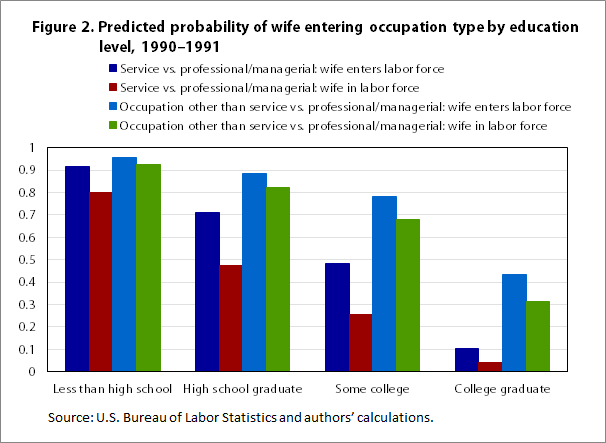
Table 6 also shows that wives with higher levels of education were more likely to work in professional or managerial occupations than in service occupations or other occupations. This is consistent with our expectations that higher levels of human capital, such as a college degree, are typically job qualifications of professionals and managers. When we compare the 1990–1991 recession with the Great Recession, we find that college graduates during the Great Recession were more likely to enter professional or managerial occupations than service or other occupations; this finding is contrary to our expectation that the severity of the Great Recession would limit college graduates’ ability to gain employment in line with their qualifications. Figures 1–3 show predicted probabilities by educational attainment for wives who were already working and for wives who started a job during the recession for each recession analyzed. These figures suggest that female college graduates who entered the labor force during the Great Recession were somewhat more likely to enter service occupations than professional occupations and were more likely to enter other occupations compared with professional occupations than their counterparts who were already in the labor force. However, this latter pattern is most evident during the Great Recession and the recession of 1990–1991, suggesting the possibility that wives were entering occupations for which they were overqualified during recession (models available upon request). Figures 1–3 also show declines over time in wives’ likelihood of entering service or other occupations, as we expect given female rising education.
WE BEGAN THIS ARTICLE with three research questions. First, we considered whether wives who were not working or seeking work at first observation were more likely to enter the labor force if their husband stopped working during the Great Recession compared with the 1990–1991 recession and the 1981–1982 recession. Our results suggest that a husband’s stopping work is associated with a higher likelihood that a wife entered the labor force during all three recessions, but that the effect was stronger during the Great Recession than in the 1981–1982 recession.
Second, we broke the outcome variable down to determine if a wife who was not in the labor force when her husband stopped working was a) more often finding a job (becoming employed) and b) more often seeking a job (becoming unemployed) than were other wives who were not in the labor force. A wife whose husband stopped working was more likely to find work than were other wives previously outside of the labor force during the Great Recession and during the 1990–91 recession. However, during the 1981–1982 recession, such wives were actually less likely to find work. During all three recessions wives were more likely to commence a job search if their husbands stopped working. This suggests that the recessionary context may be pushing women into the labor force, but only in the two more recent recessions were such wives likely to be successful in finding a job. Further research is needed to determine why this is so. It is possible that with increased education and perhaps increased job experience, wives who were not initially in the labor force were better poised to find a job when their husbands stopped working. It is also plausible that wives were less selective about the jobs they took during the more recent recessions because of the long length of the recession, the long duration of unemployment, and its associated long-term financial pressures. Future research that considers these possibilities would advance our understanding of how couples navigate economic downturns.
Third, we explored the type of occupations wives commencing work entered and compared these with the occupations of wives who already were employed at the time of the initial data collection. We found some evidence that newly employed wives were more often in service jobs rather than professional and managerial jobs in 2008–2009 and 1990–1991, but not in 1981–1982. This is consistent with the transformation of the economy and the dramatic growth in service occupations. There are also several other possibilities: service occupations may be easier to obtain, and wives, who otherwise would only consider professional or managerial jobs, may be pushed into service jobs during time of economic strain. It is also possible that service jobs are more easily balanced with the demands of family life or that wives entering jobs were seeking temporary employment. Also, perhaps some wives seek any kind of employment so they could obtain key benefits like health insurance coverage, although service occupation workers are less likely to have health insurance coverage than workers in professional or managerial jobs.52 Finally, if these wives see their employment as temporary and lasting just until their husbands resume working, service occupations may be an attractive option. Qualitative research could help us gain leverage on the answers to these questions.
One limitation of our study is that the CPS does not track people who relocate. In the context of a recession with both higher than average foreclosures and frozen housing markets, it is unclear whether those same families experiencing a husband’s job loss are more or less apt to move. Another limitation is the short window of observation. We can analyze employment status at two time points that are a year apart. However, we do not know what happened in the preceding or following months. Thus a wife who is unemployed in May may have commenced work the following month, in June. Similarly, we do not know the precise dates when husbands stopped working and when wives started. However, even if a wife entered the labor force within the same year but in advance of when her husband stopped working, it is plausible that the ending of his work was anticipated or facilitated by her employment. Our analysis is also limited in that the May CPS data do not include variables measuring personal earnings; thus, we cannot assess the extent to which a wife’s earnings make up for lost earnings of her husband or help keep the family out of poverty when faced with a husband’s job loss. Future research on the added-worker effect would do well to analyze longitudinal data with these limitations in mind.
Our research points to the possibility that wives entering employment during the Great Recession and the 1990–1991 recession may have been less particular about the jobs they took, a pattern that holds even for college graduates. This finding has implications for gender equality and lifetime earnings. Women who otherwise would have entered more lucrative jobs but instead entered lower paying service jobs, for whatever reason, will have lower earnings in the short-term and reduced lifetime earnings and pension benefits, and these reductions contribute to an increase in the gender wage gap.53 However, future research is needed to determine if the occupational patterns found during recessions are typical entry points for women when they return to work regardless of business cycle, and whether the “on ramps” for women differ by education in nonrecession years. This is beyond the scope of this paper but is an important next step.
Category | May 2008–2009 | May 1990–1991 | May 1981–1982 | |||
|---|---|---|---|---|---|---|
| Coefficient | Standard error | Coefficient | Standard error | Coefficient | Standard error | |
Husband becomes not employed | 0.651 | 0.145*** | 0.515 | 0.016*** | 0.276 | 0.013*** |
Wife's characteristics | ||||||
Wife’s education | ||||||
Less than high school (reference category) | ||||||
High school graduate | -.073 | .145 | .672 | .013*** | .411 | .009*** |
Some college | .372 | .150* | .911 | .014*** | .593 | .012*** |
Bachelor’s degree or higher | .485 | .156** | .960 | .016*** | .486 | .014*** |
Wife’s age | -.032 | .005*** | -.068 | .000*** | -.048 | .000*** |
Wife’s race and ethnicity | ||||||
White, non-Hispanic (reference category) | ||||||
Black, non-Hispanic | .058 | .176 | .376 | .018*** | .515 | .015*** |
Other, non-Hispanic | -.390 | .169* | -.218 | .021*** | .210 | .025*** |
Hispanic | .034 | .127 | .038 | .016* | .035 | .015*** |
Family variables | ||||||
Number of children under age 18 | .104 | .045* | .080 | .004*** | -.057 | .004*** |
Child under age 5 | -.536 | .120*** | -.804 | .011*** | NA | |
Family income(1) | ||||||
Less than $25,000 (reference category) | ||||||
$25,000 to $49,999 | -.119 | .143 | .045 | .013*** | -.164 | .012*** |
$50,000 to $74,999 | -.001 | .151 | .156 | .014*** | .034 | .013*** |
$75,000 to $99,999 | .064 | .163 | -.083 | .015*** | -.203 | .013*** |
$100,000 or more | -.314 | .164 | -.035 | .016* | -.451 | .019*** |
Family income data missing | -.347 | .164* | .150 | .018*** | -.275 | .017 |
Region | ||||||
Northeast (reference category) | ||||||
Midwest | .091 | .132 | .095 | .013*** | .116 | .010*** |
West | -.059 | .033 | .050 | .003*** | .085 | .003*** |
South | -.104 | .118 | .204 | .012*** | .077 | .010*** |
Residence | ||||||
Rural | -.249 | .119* | .177 | .010*** | .008*** | |
Constant | -.382 | .319 | .334 | .028*** | -.169 | .021*** |
N | 2,243 | 3,150 | 4,795 | |||
df | 19 | 19 | 18 | |||
Notes: (1) For 1990–1991: less than $24,707.94, $24,709.59 to $49,417.53, $49,419.18 to $65,890.59, $65,892.24 to $97,191.05, $98,838.36 or more. For 1981–1982: less than $23,683.32, $23,685.68 to $47,368.99, $47,371.36 to $59,211.84, 59,214.20 to $118,426.04, $118,428.41 or more. * p < .05 Note: NA indicates that the data for whether a family has a child under age 5 are not available for 1981 and 1982. Source: Individual matched 2008–2009, 1990–1991, and 1981–1982 May Current Population Survey, U.S. Bureau of Labor Statistics, and authors’ calculations. | ||||||
Category | May 2008–May 2009 | May 1990–May 1991 | May 1981–May 1982 | |||||||||
|---|---|---|---|---|---|---|---|---|---|---|---|---|
| Wife becomes employed | Wife becomes unemployed | Wife becomes employed | Wife becomes unemployed | Wife becomes employed | Wife becomes unemployed | |||||||
| Coef-ficient | Standard error | Coef-ficient | Standard error | Coef-ficient | Standard error | Coef-ficient | Standard error | Coef-ficient | Standard error | Coef-ficient | Standard error | |
Husband becomes not employed | 0.384 | 0.017** | 1.285 | 0.032** | 0.459 | 0.169*** | 1.225 | 0.253** | 0.016** | 1.400 | 0.022*** | |
Wife’s characteristics | ||||||||||||
Wife’s education | ||||||||||||
Less than high school (reference category) | ||||||||||||
High school graduate | .795 | .014 | .063 | .029** | .157 | .168*** | -.753 | .282† | .484 | .010*** | .022 | .022 |
Some college | 1.002 | .015*** | .564 | .031 | .620 | .172*** | -.483 | .306*** | .710 | .012*** | -.235 | .031*** |
Bachelor’s degree or higher | 1.161 | .017*** | -.990 | .059 | .682 | .180*** | -.055 | .306*** | .517 | .015*** | .412 | .033*** |
Wife’s age | -.062 | .001*** | -.112 | .001*** | -.026 | .006*** | -.056 | .010*** | -.044 | .000*** | -.069 | .001*** |
Wife’s race and ethnicity | ||||||||||||
White, non-Hispanic (reference category) | ||||||||||||
Black, non-Hispanic | .061 | .021 | 1.637 | .032* | -.165 | .207** | .755 | .306*** | .408 | .016*** | 1.121 | .031*** |
Other, non-Hispanic | -.179 | .021* | -.563 | .073 | -.428 | .188*** | -.259 | .351*** | .257 | .026*** | -.106 | .070 |
Hispanic | -.076 | .018 | .606 | .034 | -.003 | .140*** | .133 | .271*** | -.090 | .017*** | .582 | .030*** |
Family variables | ||||||||||||
Number of children under age 18 | .102 | .005** | -.064 | .012 | .144 | .049*** | -.076 | .102*** | -.047 | .004*** | -.124 | .009*** |
Child under age 5 | -.790 | .011*** | -.877 | .028* | -.508 | .130*** | -.652 | .265*** | NA | NA | ||
Family income(1) | ||||||||||||
Less than $25,000 (reference category) | ||||||||||||
$25,000 to $49,999 | .004 | .014 | .360 | .032 | -.186 | .160 | .108 | .283*** | -.174 | .012*** | -.083 | .026** |
$50,000 to $74,999 | .168 | .015 | -.126 | .044 | .075 | .163*** | -.505 | .362** | .040 | .013** | -.034 | .031 |
$75,000 to $99,999 | -.143 | .015 | .441 | .040 | .064 | .178*** | .051 | .350*** | -.231 | .013*** | -.011 | .031 |
$100,000 or more | -.112 | .017 | .639 | .046 | -.274 | .178*** | -.597 | .381*** | -.432 | .019*** | -.898 | .064*** |
Family income data missing | .075 | .019* | .568 | .044 | -.401 | .182*** | -.170 | .334*** | -.332 | .018*** | .068 | .039† |
Region | ||||||||||||
Northeast (reference category) | ||||||||||||
Midwest | .138 | .013 | -.439 | .040 | .130 | .145*** | -.114 | .281** | .095 | .011*** | .259 | .026*** |
West | .054 | .003 | .003 | .009† | -.048 | .036*** | -.116 | .069 | .081 | .003*** | .111 | .007*** |
South | .160 | .012 | .527 | .032* | .004 | .129*** | -.594 | .261** | .094 | .011*** | -.029 | .027 |
Residence | ||||||||||||
Rural | .212 | .010 | -.161 | .028** | -.120 | .124*** | .379** | .252 | .008*** | .380 | .019*** | |
Constant | -.103 | .030*** | .015 | .065 | .357*** | -.051 | .641 | -.449 | .022*** | .048*** | ||
N | 2,243 | 3,150 | 4,795 | |||||||||
Notes: (1) For 1990–1991: less than $24,707.94, $24,709.59 to $49,417.53, $49,419.18 to $65,890.59, $65,892.24 to $97,191.05, $98,838.36 or more. For 1981–1982: less than $23,683.32, $23,685.68 to $47,368.99, $47,371.36 to $59,211.84, $59,214.20 to $118,426.04, $118,428.41 or more. † p<.10 Note: NA indicates that the data for whether a family has a child under age 5 are not available for 1981 and 1982. Source: Individual matched 2008–2009, 1990–1991, and 1981–1982 May Current Population Survey, U.S. Bureau of Labor Statistics, and authors’ calculations. | ||||||||||||
Kristin E. Smith and Marybeth J. Mattingly, "Husbands’ job loss and wives’ labor force participation during economic downturns: are all recessions the same?," Monthly Labor Review, U.S. Bureau of Labor Statistics, September 2014, https://doi.org/10.21916/mlr.2014.31
1 According to the National Bureau of Economic Research, this recession began in December 2007 and ended in June 2009.
2 Losses in investments are discussed in John Irons, “Economic scarring: the long-term impacts of the recession,” EPI briefing paper no. 243 (Washington, D.C.: Economic Policy Institute, 2009). The reduction in the availability of credit is discussed in Randy Albelda and Christa Kelleher, “Women in the down economy: impacts of the recession and the stimulus in Massachusetts,” policy brief, The Center for Women in Politics and Public Policy, the Center for Social Policy, and the Massachusetts Commission on the Status of Women, March 2010.
3 David B. Grusky, Bruce Western, Christopher Wimer, eds., The Great Recession (New York: Russell Sage Foundation, 2011).
4 Henry S. Farber, “Job loss in the Great Recession: historical perspective from the Displaced Workers Survey,” 1984–2010, NBER working paper no. 17040 (Washington, DC: National Bureau of Economic Research, May 2011).
5 Jeffrey K. Liker and Glen H. Elder, Jr., “Economic hardship and marital relations in the 1930s,” American Sociological Review 48, 1983, pp. 343–359.
6 Sarah B. Raley, Marybeth J. Mattingly, and Suzanne M. Bianchi, “How dual are dual-income couples? Documenting change from 1970 to 2001,” Journal of Marriage and Family, February 2006, pp. 11–28.
7 Kristin E. Smith, “Changing Roles: Women and Work in Rural America,” in Kristin E. Smith and Ann R. Tickamyer, eds., Economic restructuring and family well-being in rural America (University Park: Pennsylvania State University Press, 2011), pp. 60–81.
8 Reasons for stopping work include losing a job, leaving a job, retirement, and on temporary layoff. Marybeth J. Mattingly and Kristin E. Smith, “Changes in wives’ employment when husbands stop working: a recession–prosperity comparison,” Family Relations, October 2010, pp. 343–357.
9 Ibid.
10 Carmen DeNavas-Walt, Bernadette D. Procter, and Jessica C. Smith, Income, poverty, and health insurance coverage in the United States: 2010, Current Population Reports P60-239 (U.S. Census Bureau, 2011).
11 Kristin E. Smith and Andrew Schaefer, “Families continue to rely on wives as breadwinners post-recession: an analysis by state and place type,” Issue Brief 75 (Durham, NH: Carsey Institute, University of New Hampshire, 2014).
12 Melvin Stephens, Jr., “Worker displacement and the added worker effect,” Journal of Labor Economics, vol. 20, issue 3, 2002, pp. 504–537.
13 Mattingly and Smith, “Changes in wives’ employment.”
14 Rand D. Conger and Glen H. Elder, Jr., Families in troubled times: adapting to change in rural America (New York: Aldine De Gruyter, 1994).
15 Wei-Jun JeanYeung and Sandra L. Hofferth, “Family adaptations to income and job loss in the U.S.,” Journal of Family and Economic Issues, vol. 19, issue 3, 1998, pp. 255–283.
16 Orley Ashenfelter and James J. Heckman, “The estimation of income and substitution effects in a model of family labor supply,” Econometrica, January 1974, pp. 73–85.
17 Carolyn M. Moehling, “Women's work and men's unemployment,” Journal of Economic History, March 2001, pp. 926–949.
18 Shelly Lundberg, “The added worker effect,” Journal of Labor Economics, vol. 3, issue 1, 1985, pp. 11–37.
19 BBC News, “Timeline: credit crunch to downturn,” August 7, 2009, http://news.bbc.co.uk/2/hi/7521250.stm.
20 Lundberg, “The added worker effect;” Doki K. Tano, “The added worker effect: a causality test,” Economics Letters, vol. 43, issue 1, 1993, pp.111–17; Yeung and Hofferth, “Family adaptations to income and job loss.”
21 Tim Maloney, “Unobserved variables and the elusive added worker effect,” Economica, vol. 58, issue 230, 1991, pp. 173–187; Chinhui Juhn and Kevin M. Murphy, “Wage inequality and family labor supply,” NBER working paper no. 5459 (Cambridge, MA: National Bureau of Economic Research, February 1996).
22 Mattingly and Smith, “Changes in wives’ employment;” Liana C. Landivar, “The impact of the Great Recession on mothers’ employment,” in Sampson Lee Blair, ed., Economic stress and the family, Contemporary Perspectives in Family Research, vol. 6, 2012, pp. 163–185; Martha A. Starr, “Gender, added-worker effects, and the 2007–2009 recession: looking within the household,” Review of Economics of the Household, June 2014, pp. 209–235.
23 Recession start and end dates are determined by the National Bureau of Economic Research. See “US business cycle expansions and contractions” at http://www.nber.org/cycles/cyclesmain.html. Also see Kevin L. Klieson, “The 2001 recession: how was it different and what developments may have caused it?” The Federal Reserve Bank of St. Louis Review, September/October 2003.
24 Calculated from the Current Employment Statistics Survey data, U.S. Bureau of Labor Statistics, https://www.bls.gov/ces/; Rakesh Kochar, “Two years of economic recovery: women lose jobs, men find them,” Social and Demographic Trends, Pew Research Center, July 6, 2011.
25 Calculated from Current Population Survey data in “Table A-1. Employment status of the civilian population by sex and age,” 2011, U.S. Bureau of Labor Statistics, https://www.bls.gov/webapps/legacy/cpsatab1.htm.
26 Ibid.
27 Calculated from Current Population Survey data in “Table A-12. Unemployed persons by duration of unemployment,” 2011, U.S. Bureau of Labor Statistics, https://www.bls.gov/webapps/legacy/cpsatab12.htm; Michael A. Urquhart and Marillyn A. Hewson, “Unemployment continued to rise in 1982 as recession deepened,” Monthly Labor Review, February 1983, https://www.bls.gov/opub/mlr/1983/02/art1full.pdf.
28 Calculated from Current Employment Statistics Survey data, U.S. Bureau of Labor Statistics, https://www.bls.gov/ces/.
29 Cynthia J. Brown and Jose A. Pagan, “Changes in employment status across demographic groups during the 1990–1991 recession, Applied Economics, vol. 30, issue 12, 1998, pp. 1,571–1,583; Klieson, “The 2001 recession.”
30 Timothy Parker, Lorin Kusmin, and Alexander Marré, “Economic recovery: lessons learned from previous recessions,” Amber Waves, March 2010, U.S. Department of Agriculture Economic Research Service.
31 Calculated from Current Employment Statistics Survey data, U.S. Bureau of Labor Statistics, https://www.bls.gov/ces/.
32 Robert Drago and Claudia Williams, “The gender wage gap: 2009,” Fact Sheet, IWPR #C350 (Washington, DC: Institute for Women’s Policy Research), September 2010, http://www.iwpr.org/publications/pubs/the-gender-wage-gap-2009. The annual estimates are derived from annual earnings data from the Current Population Survey.
33 Mattingly and Smith, “Changes in wives’ employment.”
34 During the recovery, however, government sector jobs have been lost as states face lower revenues and the federal government stimulus money ceased, leaving more women unemployed in the wake of the recession. From Kochar, “Two years of economic recovery.”
35 Kristin Smith, Kristin and Ann R. Tickamyer, eds., Economic restructuring and family well-being in rural America (University Park, PA: Pennsylvania State University Press, 2011).
36 William E. Even and David A. Macpherson, “The decline of private-sector unionism and the gender wage gap,” Journal of Human Resources, Spring 1993, pp. 279–296.
37 David A. Cotter, Joan M. Hermsen, and Reeve Vanneman, Reeve, “Gender inequality at work” (New York: Russell Sage Foundation, 2004); Paula England, “Reassessing the uneven gender revolution and its slowdown,” Gender & Society, February 2011, 113–123.
38 Jennifer Tomlinson, Wendy Olsen, and Kingsley Purdam, “Women returners and potential returners: employment profiles and labour market opportunities – a case study of the United Kingdom,” European Sociological Review, vol. 25, issue 3, 2009, pp. 349–363.
39 Pamela Stone, Opting out? Why women really quit careers and head home (Berkeley, CA: University of California Press, 2007).
40 Paula England, “Gender inequality in labor markets: the role of motherhood and segregation,” Social Politics, vol. 12, issue 2, 2005, pp. 264–288.
41 Tomlinson, Olsen, and Purdam, “Women returners and potential returners.”
42 Mattingly and Smith, “Changes in wives’ employment.”
43 Teresa Amott and Julie Matthaei, Race, gender, and work: a multicultural economic history of women in the United States (Boston, MA: South End Press, 1991).
44 Julie Berry Cullen and Jonathan Gruber, “Does unemployment insurance crowd out spousal labor supply?” Journal of Labor Economics, July 2000, pp. 546–572.
45 U.S. Census Bureau, Current Population Survey, May 2008 and May 2009 data.
46 In this article, we use the term entering the labor force to indicate whether a wife was neither employed nor seeking work at time 1 (e.g., May 2008) but was employed or seeking work at time 2, one year later (e.g., May 2009). It is possible that wives entered the labor force and then exited within the 1-year time period and we would not capture them as entering the labor force.
47 Raymond Paternoster, Robert Brame, Paul Mazerolle, and Alex Piquero, “Using the correct statistical test for the equality of regression coefficients,” Criminology, November 1998, pp. 859–866.
48 Philip N. Cohen and Suzanne M. Bianchi, “Marriage, children, and women’s employment: what do we know?” Monthly Labor Review, December 1999, 22–31.
49 U.S. Bureau of Labor Statistics, Local Area Unemployment Statistics, https://www.bls.gov/sae/#data.
50 Even and Macpherson, “The decline of private-sector unionism.”
51 Calculated from Current Employment Statistics Survey data, U.S. Bureau of Labor Statistics, https://www.bls.gov/ces/.
52 Sharon A. DeVaney and Sophia T. Anong, “The likelihood of having employer-sponsored health insurance,” Monthly Labor Review, November 2007.
53 Michelle J. Budig and Paula England, “The wage penalty for motherhood,” American Sociological Review, April 2001, pp. 204–225; Mariko Lin Chang, Shortchanged: why women have less wealth and what can be done about it (NY: Oxford University Press, 2010).