An official website of the United States government
An official website of the United States government
The .gov means it's official.
Federal government websites often end in .gov or .mil. Before sharing sensitive information,
make sure you're on a federal government site.
The site is secure.
The
https:// ensures that you are connecting to the official website and that any
information you provide is encrypted and transmitted securely.
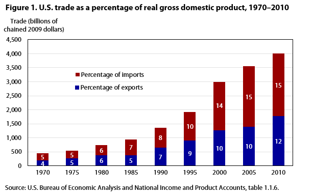
Over the past four decades, international trade has made a growing contribution to U.S. economic activity. Figure 1 shows that trade in goods and services increased from $441 billion in 1970 to nearly $4 trillion in 2010. As a percentage of gross domestic product (GDP), trade’s share has tripled since 1970 to 27 percent of GDP in 2010.
The GDP, published by the U.S. Bureau of Economic Analysis (BEA), is considered the most comprehensive measure of economic activity in the United States. Decisionmakers in both the government and the private sector widely follow the GDP. The U.S. Bureau of Labor Statistics (BLS) role in the creation of this important economic measure is essential. This article describes the U.S. import and export price indexes published by the BLS International Price Program (IPP). In addition, it explains how BEA uses these indexes to calculate the trade component of real GDP and two related measures of international competitiveness.
The GDP is the most comprehensive measure of the output of final goods and services produced in the United States and is one of the most closely watched economic statistics in the world.1 A general representation of GDP is as follows:
GDP = consumption + government expenditures + investments + (exports – imports)
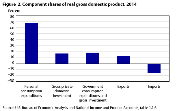
This article focuses on the foreign-trade component of GDP, also known as “net exports” (exports less imports), and the method in which BEA uses the IPP U.S. import and export price indexes to adjust for inflation. Net exports measure the impact of the foreign-trade sector on the economy. If exports outweigh imports, then the foreign-trade sector has a positive contribution to GDP. Conversely, if imports outweigh exports, as is the current situation in the United States, then the foreign-trade sector has a negative contribution to GDP. Figure 2 shows how trade (exports and imports) compares with the other components of GDP in terms of contribution to total GDP.
The IPP was created in the early 1970s to develop the statistics necessary to calculate inflation-adjusted measures of merchandise trade and GDP. The IPP published its first annual price indexes in 1973 and first quarterly indexes in 1974.2 The Office of Management and Budget placed the IPP indexes on its list of Principal Federal Economic Indicators in 1982. By 1989, the IPP began publishing a limited number of monthly price indexes. Later that year, the U.S. Census Bureau (Census) began using the IPP U.S. import and export price indexes to deflate merchandise trade statistics.3 In 1993, the IPP began publishing all indexes monthly.
The import price indexes measure the monthly changes in the prices of goods and services that U.S. residents purchase from foreign suppliers. The export price indexes measure the monthly changes in the prices of goods and services that U.S. residents sell to foreign buyers. Currently, the IPP publishes over 1,000 indexes each month that cover nearly all U.S. foreign trade in goods and two categories of transportation services (airfreight and air passenger fares). Some indexes measure the price change for a broad category, such as all exports, while other indexes measure the price change for more specific commodities, such as corn exports. The IPP publishes the indexes at the lowest level of detail possible while meeting index quality criteria, such as adequate item coverage and response rates.4
The IPP publishes import and export price indexes for merchandise trade on the basis of three major classification systems:
1. The BEA end use, which is the system that Census and BEA use to construct the foreign-trade portion of the national income and product accounts (NIPA)5
2. The North American Industry Classification System, which government statistical agencies in the United States, Canada, and Mexico jointly developed to allow for greater comparability of business statistics among the North American economies6
3. The Harmonized System, which is based on a commodity classification system that the World Customs Organization developed and the U.S. International Trade Commission maintains in the United States to apply tariffs7
The IPP locality of origin indexes measure the monthly changes in the prices of goods imported from 15 countries and regions. The IPP also publishes indexes covering two categories of transportation services.
BLS uses a modified form of the Laspeyres index to calculate the IPP import and export price indexes. One feature of the IPP index calculation is that the quality of items is fixed so the indexes capture pure price changes and not quality changes. For example, if the import price of a computer processor increases solely because of an increase in its processing speed while all other factors remain the same, then the new price will be adjusted to show no change from the previous month.8
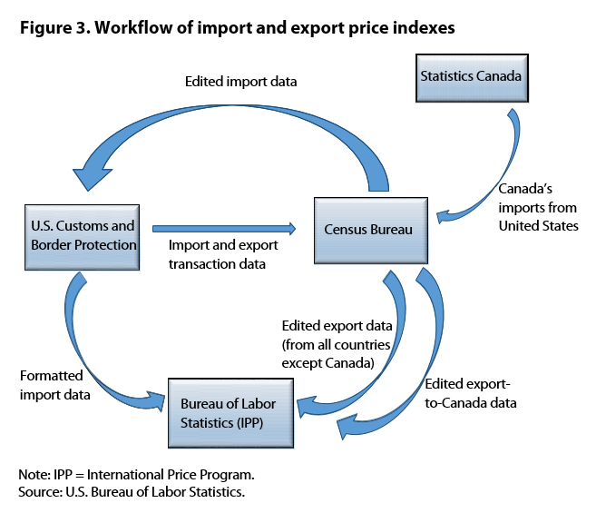
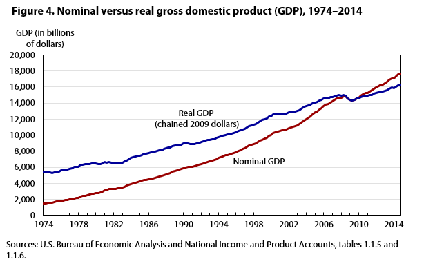
Figure 3 outlines the basic flow of data among the agencies involved in producing the import and export data used to create the import and export price indexes and eventually deflate GDP. First, U.S. Customs and Border Protection (Customs) collects data on import and export transactions. Customs collects many data points on each transaction, a few of which include country, Harmonized System classification number, and dollar value. Second, Customs sends the transaction data to Census for further processing and editing. Third, after processing the import transactions data, Census returns the data to Customs, which formats and sends the data to the IPP. For exports, Census sends the export data directly to the IPP after processing and editing. Statistics Canada sends data to Census on Canada’s imports from the United States. Census sends these data to the IPP to use for U.S. exports to Canada.
The import and export price indexes are important in the government statistical community and for government policymakers, private business, and academia. One essential function of the import and export price indexes is adjusting the foreign-trade portion of GDP and monthly merchandise trade statistics for inflation, both of which are released by the Department of Commerce. Government officials in charge of monetary policy also use import price indexes to gauge the impact of exchange rate fluctuations on the prices of imported goods, which can affect the prices of domestic output.9 Private companies use import and export price indexes for contract escalations. For example, when a U.S. producer contracts with a foreign supplier, the contract can stipulate that the U.S. producer will change how much it will pay the supplier for a certain input, such as steel rebar. The U.S. producer determines this payment change on the basis of the movement of an IPP import price index that closely relates to that input. Finally, academic researchers use import and export price indexes to investigate many economic issues, such as the competitiveness of U.S.-produced versus foreign-produced goods and how fluctuations in exchange rates affect U.S. consumers.
The BEA publishes GDP in both nominal and real terms. With nominal, or current-dollar GDP, the BEA estimates the dollar value of output in a given quarter without adjusting for inflation. Nominal GDP does not clearly show whether the change is a result of the quantity of goods and services output or is due to a change in the price of those goods and services. Real GDP, however, more clearly shows how the economy is performing over a long period because the effect of price changes is removed. BEA calculates real GDP by dividing the nominal value by an appropriate price index, thereby removing the effect of inflation. Figure 4 shows how real GDP grows over the period at a slower rate than the rate for nominal GDP because the effect of price fluctuations is removed.
Because GDP is a very broad measure of activity, an example of a specific component can help show how real and nominal series can move differently. For example, a severe drought hit the U.S. Corn Belt in the summer of 2012, sending the price index for exported corn to the highest recorded level since BLS began measuring monthly export prices.10 Corn is a major export crop for the United States and is the largest contributor to the U.S. trade surplus in agricultural goods.11
Table 1 shows how the real export value eliminates the effect of price changes for corn exports during the period from June through August 2012. The nominal value of corn exports, as reported by the BEA, decreased throughout the period, but the price level of corn increased, which provides more information about the underlying economic activity.12 Therefore, the increasing price of corn held the nominal export value “artificially” high. The real value of corn exports decreased much more than the nominal value, which clearly shows the underlying economic activity: the volume of exports (i.e., bushels of corn exported) decreased much more rapidly than the nominal value of exports suggested.
| Month | Nominal corn export value (millions of dollars) | Corn export price index | Rebased export corn price index | Real corn export value (millions of dollars) | Difference between real and nominal corn exports (millions of dollars) |
|---|---|---|---|---|---|
| June | $926 | 277.1 | 100.0 | $926.00 | $0 |
| July | 809 | 330.4 | 119.2 | 678.70 | –130.30 |
| August | 733 | 367.1 | 132.5 | 553.20 | –179.80 |
| Sources: U.S. Bureau of Labor Statistics and U.S. Bureau of Economic Analysis. | |||||
Price indexes are based to a specific period, which varies from index to index. To convert a nominal series to a real series, one must rebase the price index to correspond to the period examined. In table 1, the export price index of corn is rebased by dividing each month’s price index level by June’s price index level (277.1). In other words, the rebased price index levels for each month are set in terms of June prices.
The real export value of corn is computed using equation (1) as follows
Real export value = (Nominal export value/Rebased price index) × 100 (1)
Why are the IPP import and export price indexes the most appropriate for deflating net exports? Currently, no other statistics exist that measure prices of goods imported into or exported from the United States.13 As such, the import and export price indexes the IPP produces are essential in deflating the net exports portion of GDP.14
As mentioned earlier, BLS publishes import and export price indexes using the BEA end-use classification system, which the BEA uses to deflate the foreign transactions sector of GDP. The BEA NIPA tables provide a wealth of data that underlie the final headline GDP figure. In addition, NIPA tables provide the general process of how the BEA uses the IPP import and export indexes to deflate foreign transactions. For example, the NIPA tables show how BEA uses the IPP export price indexes to deflate exports of foods, feeds, and beverages. The third line of the NIPA table 4.2.5 contains the nominal value for exports of foods, feeds, and beverages.15 For the third quarter of 2012, the total was $148 billion.16 NIPA table 4.2.4 contains the price indexes that correspond to the BEA end-use categories for goods, as well as to various categories of services. The IPP import and export price indexes are a prominent input to this table, especially in the categories of goods. In NIPA table 4.2.4, the price index value for the third quarter of 2012 for exports of foods, feeds, and beverages was 135.58. As shown in equation (1), to calculate a real value, divide the nominal value (NIPA table 4.2.5) by the price index (NIPA table 4.2.4) and multiply by 100. Applying the equation to the example for exports of foods, feeds, and beverages shows that the real value for the third quarter of 2012 is $109.2 billion, which is published in NIPA table 4.2.6.
The BEA uses a much finer level of detail of the IPP import and export price indexes than that which is published in the NIPA tables. The example in tables 2 and 3 uses simulated data and outlines the overall process of how the BEA uses the IPP indexes to build up from commodity-level data many of the price indexes in NIPA table 4.2.4. Although the example is for exports, the same process occurs for imports. Continuing with the example for foods, feeds, and beverages, assume that the category comprises only corn, soybean, and wheat.17
| Commodity | Month | BLS price index percent change (not seasonally adjusted) | BEA price index | Seasonally adjusted monthly trade value (millions of dollars) | Monthly trade value weight | Monthly weighted price index (seasonally adjusted) | Quarterly price index (seasonally adjusted) | |
|---|---|---|---|---|---|---|---|---|
| Not seasonally adjusted | Seasonally adjusted | |||||||
| Corn | January | 1.2 | 207 | 215 | $2 | 0.29 | 62.35 | — |
| February | 3.0 | 213 | 210 | 1 | .14 | 29.40 | — | |
| March | .8 | 215 | 220 | 4 | .57 | 125.40 | — | |
| — | — | — | — | — | — | — | 217.15 | |
| Soybeans | January | 2.0 | 214 | 210 | 5 | .38 | 79.80 | — |
| February | 1.8 | 218 | 215 | 7 | .54 | 116.10 | — | |
| March | .9 | 220 | 220 | 1 | .08 | 17.60 | — | |
| — | — | — | — | — | — | — | 213.50 | |
| Wheat | January | 1.0 | 202 | 220 | 3 | .30 | 66.00 | — |
| February | .7 | 203 | 210 | 5 | .50 | 105.00 | — | |
| March | 3.0 | 209 | 215 | 2 | .20 | 43.00 | — | |
| — | — | — | — | — | — | — | 214.00 | |
| Source: Data are simulated. | ||||||||
First, the BEA advances the not seasonally adjusted commodity-level price indexes for each month in a quarter by the percent change in the corresponding IPP price index. For example, the IPP February price index for corn increased 3 percent from January, so the BEA advances the January price index for corn by 3 percent from 207 to 213. Thus, the levels of the BEA price indexes may differ from the IPP price indexes, but they move by the same rate each month. Second, the BEA seasonally adjusts the commodity-level price indexes, if necessary.18
Next, the monthly price indexes must be converted to a quarterly price index for each commodity. To do so, the BEA weights each monthly price index by the monthly share of the quarterly value. The final commodity-level quarterly price index is the sum of the monthly trade value-weighted indexes.
Finally, the quarterly price indexes for each commodity are summed to the price index for the aggregate end-use category, which is published in NIPA table 4.2.4. As shown in table 3, this computation is done by multiplying the quarterly price index for each commodity (e.g., corn, soybeans, and wheat) by the proportion of each commodity’s quarterly trade value within the aggregate end-use category’s (e.g., foods, feeds, and beverages) quarterly trade value.
| Commodity | Seasonally adjusted quarterly trade value (millions of dollars) | Quarterly trade value weight | Quarterly price index | Quarterly weighted price index |
|---|---|---|---|---|
| Food, feeds, and beverages | — | — | — | 212.37 |
| Corn | $7 | 0.23 | 217.15 | 49.94 |
| Soybeans | 13 | .43 | 213.50 | 91.81 |
| Wheat | 10 | .33 | 214.00 | 70.62 |
| Source: Data simulated. | ||||
Because trade has grown in importance in the United States (figure 1), having statistics that measure the real purchasing power of income that the U.S. economy generates as a measure of international competitiveness is useful. The BEA produces such a statistic called command-basis GDP, and again, the IPP price indexes are essential in constructing it. Command-basis GDP measures the value of goods and services the United States can afford to purchase in the world market, in contrast with conventional GDP, which measures the value of goods and services the U.S economy produces. Command-basis GDP is calculated similarly to conventional GDP, except that the value of exports is deflated by a price index that includes the IPP import price indexes as opposed to the IPP export price indexes.19
A statistic that has grown in importance along with the increased amount of trade is called “terms of trade” an is another measure of international competitiveness. The terms of trade statistic measures the relationship between the prices U.S. producers receive for their exports and the prices U.S. purchasers pay for their imports. The ratio of an export price index to the import price index can represent terms of trade. Thus, if the U.S. export price index increases, all else equal, then imports are cheaper in terms of exports. As a result, the United States would have to export less to import the same amount of goods and services.
This article has shown how the IPP import and export price indexes are critical in providing policymakers, researchers, and the public with an inflation-adjusted measure of GDP, which provides the most comprehensive view of economic activity in the United States. In addition, when trade comprises an increasing share of economic activity in the United States, the IPP import and export price indexes allow the BEA to derive important measures of competitiveness, such as command-basis GDP and terms of trade.
Guadalupe Cerritos, "The role of BLS import and export price indexes in the real GDP," Monthly Labor Review, U.S. Bureau of Labor Statistics, June 2015, https://doi.org/10.21916/mlr.2015.19
1 For a brief history of GDP and an overview of how it is measured, see J. Steven Landefeld, Eugene Seskin, and Barbara Fraumeni, “Taking the pulse of the economy: measuring GDP,” Journal of Economic Perspectives, Spring 2008, pp. 193–216.
2 “International price indexes,” BLS Handbook of Methods (U.S. Bureau of Labor Statistics, April 1997), chapter 15, https://www.bls.gov/opub/hom/ho mch15_a.htm.
3 For more information on how the U.S. Census Bureau uses the International Price Program U.S. import and export price indexes to deflate merchandise trade statistics, see “Adjustment of U.S. merchandise trade data for price change” (U.S. Census Bureau, Foreign Trade Division, March 2004), https://www.census.gov/foreign-trade/aip/priceadj.html.
4 For example, the International Price Program (IPP) publishes the end-use export index other agricultural goods (Q003) with five indexes below it that offer details on more specific product groups, such as meat, poultry, and other edible animal products (Q00300), and vegetables and vegetable preparations and juices (Q00320). To ensure data quality for these lower level indexes, the IPP requires that a certain number of companies submit prices each month and a certain number of items have prices updated.
5 For the current list of end-use categories, see https://www.census.gov/foreign- trade/reference/codes/enduse/imeumstr.txt for imports and https://www.census.gov/foreign- trade/reference/codes/enduse/exeumstr.txt for exports.
6 For more information on the North American Industry Classification System, see https://www.census.gov/eos/www/naics/.
7 The U.S. Census Bureau maintains the codes used for exports, which are based on the import codes that the United States International Trade Commission developed. For exports, see https://www.census.gov/foreign-trade/schedules/b/index.html.
8 For additional information on the International Price Program quality adjustment practices, see https://www.bls.gov/mxp/ippfaq.h tm#item13 and the pricing section of BLS Handbook of Methods, https://www.bls.gov/opub/hom/.
9 Etienne Gagnon, Benjamin R. Mandel, and Robert J. Vigfusson, “Missing import price changes and low exchange rate pass-through,” Federal Reserve Bank of New York Staff Reports, no. 537, January 2012, revised July 2012, http://www.ne wyorkfed.org/research/staff_reports/sr537.pdf.
10 The main corn-growing region of the United States includes Iowa, Illinois, Nebraska, Minnesota, Indiana, Wisconsin, South Dakota, Michigan, Missouri, and Kansas. For more information on the direct impacts of the drought on corn prices, see Will Adonizio, Nancy Kook, and Sharon Royales, “Impact of the drought on corn exports: paying the price,” Beyond the Numbers: Global Economy, vol. 1, no. 17, November 2012, https://www.bls.gov/opub/btn/volume-1/impact-of- the-drought-on-corn-exports-paying-the-price.htm.
11 See “U.S. corn trade” (U.S. Department of Agriculture, Economic Research Service, January 15, 2015), http://www.ers.usda .gov/.
12 For detailed goods trade data, see “International accounts products for detailed goods trade data: U.S. trade in goods (IDS-0182)” (U.S. Department of Commerce, Bureau of Economic Analysis, June 5, 2015), http://www.bea. gov/international/detailed_trade_data.htm.
13 For a detailed discussion on why the International Price Program indexes are the most appropriate for measuring export prices, see Bill Alterman, “Are producer prices good proxies for export prices?” Monthly Labor Review, October 1997, pp. 18–32, https://www.bls.gov/mlr/1997/ 10/art3full.pdf.
14 See the “Net exports of goods and services,” National Income and Product Accounts Handbook (U.S. Department of Commerce, Bureau of Economic Analysis, November 2014), chapter 8, pp. 8-17–8-23, https://apps.bea.gov/national/pdf/chapter8.pdf.
15 The NIPA tables are available at “National data, GDP & personal income” (U.S. Department of Commerce, Bureau of Economic Analysis), https://apps.bea.gov/iTable/index_nipa.cf m.
16 Note that the Bureau of Economic Analysis publishes most dollar-value data seasonally adjusted to annual rates. A discussion of annual rates is beyond the scope of this article.
17 Wheat, soybeans, and corn together make up 34 percent of the weight for the International Price Program foods, feeds, and beverages end-use export price index (based on 2012 trade weights).
18 Seasonal adjustment is a statistical technique that removes seasonal variations from economic data series that occur in the same month or quarter each year (e.g., consumer spending, which increases every December and decreases every January). Seasonally adjusted data series better reflect economic trends that are not linked to recurring economic activity.
19 For command-basis gross domestic product (GDP), the Bureau of Economic Analysis uses the gross domestic purchases price index to deflate both exports and imports. For more information on command-basis GDP, see System of National Accounts, 2008 (United Nations and World Bank, 2009), paragraph 15.188, http://unsta ts.un.org/unsd/nationalaccount/docs/SNA2008.pdf. The System of National Accounts refers to command-basis GDP as real gross domestic income, but the concept is identical.